Learning Lab

Range

To compare data sets it is also useful to look at the measure of spread.

The most basic measure of spread is the range, the distance from the smallest to the largest value.

Set A \[\begin{align*} \text{Range} & =\text{highest value$-\text{lowest value}$ }\\ & =6-4\\ & =2. \end{align*}\]

Set B

\[\begin{align*} \text{Range} & =\text{highest value$-\text{lowest value}$ }\\ & =9-1\\ & =8. \end{align*}\]

We can see that Set B has greater spread than Set A. But the problem with the range is that it uses only two of the values in the data set. One of these may be an odd or unusual value called an outlier.

Consider the two sets of values below:

Set Y: \(1,1,2,2,2,2,2,100\).

Set Z: \(1,18,23,41,59,63,87,100\).

The range for both is 99 because Set Y has one unusual value - the 100. Most of the data are ones or twos. The value of 100 is unusual and is an outlier.

Interquartile Range

The Interquartile Range (IQR) is the distance between the first quartile Q\(_{1}\) and the third quartile Q\(_{3}\).

IQR = Q\(_{3}-\) Q\(_{1}\)

The first and third quartiles are values that are \(1/4\) and \(3/4\) of the way through the ordered data. Q\(_{1}\) is the median of the lower half of the data and Q\(_{3}\) is the median of the upper half of the data.

(Note: there are other ways to find Q\(_{1}\) and Q\(_{3}\) so check with your teacher.)

Set Y: \(\quad1\quad\underbrace{1\quad\downarrow\quad2}_{\text{Q$_{1}$ }}\quad2\quad\mathbf{\downarrow}\quad2\quad\underbrace{\mathbf{\mathrm{2}\quad\downarrow}\quad2}_{\text{Q$_{3}$ }}\quad100\)

The arrows indicate the location of the quartiles and \[\begin{align*} \text{Q$_{1}$ } & =\frac{1+2}{2}\\ & =1.5\\ \text{Q$_{3}$ } & =\frac{2+2}{2}\\ & =2. \end{align*}\] Hence the interquartile range is IQR = Q\(_{3}-\) Q\(_{1}\) = 2 – 1.5 = 0.5.

Now consider the other set of data:

Set Z: \(\quad1\quad\underbrace{18\quad\downarrow\quad23}_{\text{Q$_{1}$ }}\quad41\quad\mathbf{\downarrow}\quad59\quad\underbrace{\mathbf{\mathrm{63}\quad\downarrow}\quad87}_{\text{Q$_{3}$ }}\quad100\)

We have \[\begin{align*} \text{Q$_{1}$ } & =\frac{18+23}{2}\\ & =20.5\\ \text{Q$_{3}$ } & =\frac{63+87}{2}\\ & =75. \end{align*}\] Hence the interquartile range is

IQR = Q\(_{3}-\) Q\(_{1}=75-20.5=54.5\)

So for the data sets Y and Z the mean together with the IQR are better summaries of the data sets than the range.

Standard Deviation

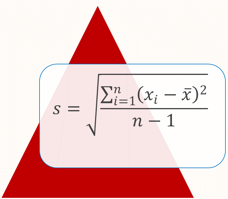
A measure of dispersion or spread in a data set that takes into account all of the data is the standard deviation. It gives an indication of the typical or average distance of each score from the mean for the data. The standard deviation can be calculated using the formula \[ s=\sqrt{\frac{\Sigma(x-\overline{x})^{2}}{n-1}} \] but it is much more convenient to use your calculator or the computer.

Some statistical tests make use of the variance which is the square of the standard deviation:

\[ \text{Variance $=$ }s^{2}=\frac{\Sigma(x-\overline{x})^{2}}{n-1}. \]

Set A:\(\quad4\quad4\quad5\quad5\quad5\quad6\quad6\)

\(\overline{x}=5\)

\(s=0.82\)

Set B: \(\quad1\quad3\quad4\quad5\quad6\quad7\quad9\)

\(\overline{x}=5\)

\(s=2.65\)

We can interpret the standard deviation: the scores in set A are typically \(0.82\) away from the mean, but the scores in set B are typically \(2.65\) away from the mean. Though set A and B have the same centre, those in set B are clearly more dispersed or have greater spread than set A.