Linear motion is how an object moves in a straight line. To describe these motions, we need to know some technical terms like displacement, distance, velocity, speed and acceleration, and how to represent how they change over time. Use this resource to learn about the terms and their relationships to one another.
In linear motion, these quantities help us describe not just how far something moves, but how fast it moves and how its motion changes over time. Let's define each quantity and show how they are connected when an object travels in a straight line.
Displacement \(\left(x\right)\)
When an object is moved from one point to another, it is said to be displaced. If we start in Melbourne and travel to Dandenong, we can say that we have been displaced \(32\,\text{km}\) from Melbourne. To then define our position, we need to specify a direction: we are \(32\,\text{km}\) South East of Melbourne. That is, we give a magnitude \(\left(32\,\text{km}\right)\) and a direction (South East). This makes position, or displacement, a vector quantity. Displacement is often used to show the position of a something relative to a specific point.
In physics, we assign a positive sign to a specific direction. For example, if East is the positive direction, then travelling \(2\,\text{km}\) East is \(+2\,\text{km}\). This would make travelling \(2\,\text{km}\) West, \(-2\,\text{km}\).
Distance \(\left(d\right)\)
Distance is the magnitude (or size) of the displacement. It is the length of the path taken by something. It has no direction, so it is a scalar quantity. For example, you can say your distance is \(60\,\text{km}\) away, but your displacement would be \(60\,\text{km}\) in a direction, such as \(60\,\text{km}\) West.
Velocity \(\left(v\right)\)
Velocity is the rate of change of displacement, \(x\). That is, for an object moving at constant velocity:
\[v=\frac{x}{t}\]
where \(t\) is the time taken.
Since displacement is a vector quantity, so is velocity.
The units of velocity depend on the units of displacement and time. If displacement is in metres \(\left(\text{m}\right)\) and time is in seconds \(\left(\text{s}\right)\), the unit of velocity is metres per second \((\text{m/s}\) or \(\text{m}\,\text{s}^{-1})\).
Speed
The speed of an object is the magnitude of its velocity. It can also be calculated by:
\[\text{speed}=\frac{d}{t}\]
where \(t\) is the time taken.
It has no direction, making it a scalar quantity.
Acceleration \(\left(a\right)\)
Acceleration is the rate of change of velocity:
\[a=\frac{v}{t}\]
If \(v\) is in metres per second, the unit of acceleration is metres per second per second: \(\text{m/s}^{2}\) or \(\text{m}\,\text{s}^{-2}\). Since velocity is a vector quantity, so is acceleration. If acceleration is constant, we use the expression 'the acceleration is uniform'.
Representing linear motion
We can describe linear motion using graphs that show how displacement, velocity and acceleration change over time.
Distance vs time graphs
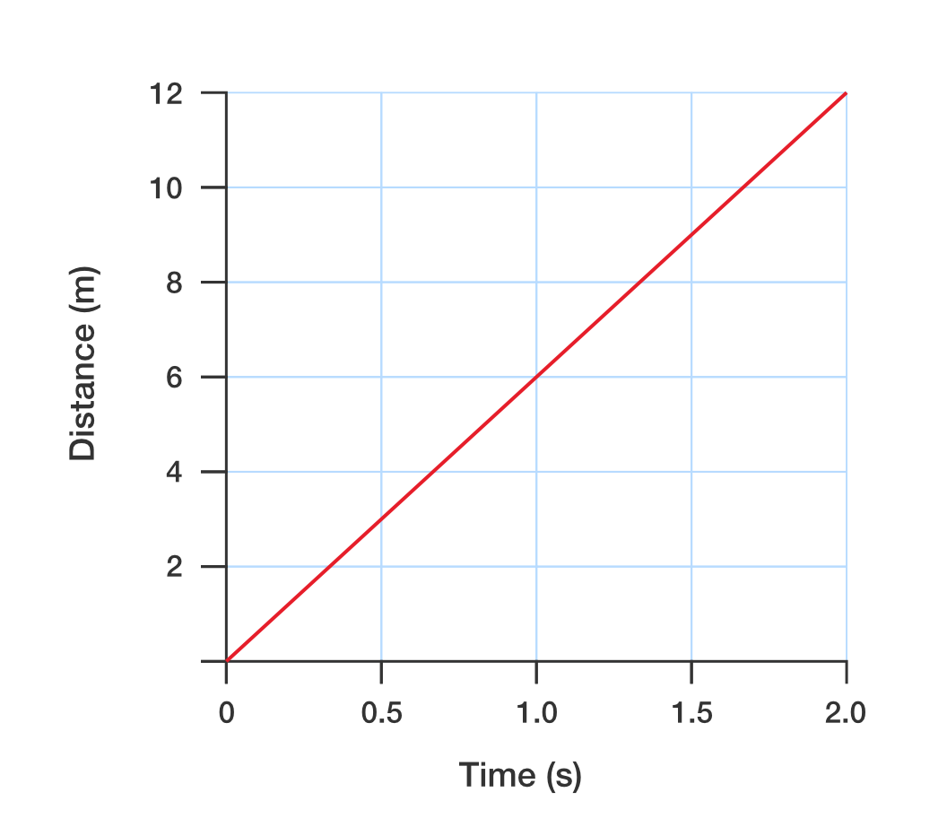
Let’s suppose a person, starting from rest, runs a distance \(d\) of \(12\,\text{m}\) in a time \(t\) of \(2\,\text{s}\). Assuming that their speed is constant, the distance–time graph would look like this:
The gradient of a distance (a scalar quantity) versus time graph gives the speed (also a scalar quantity). In this case, the speed is given by:
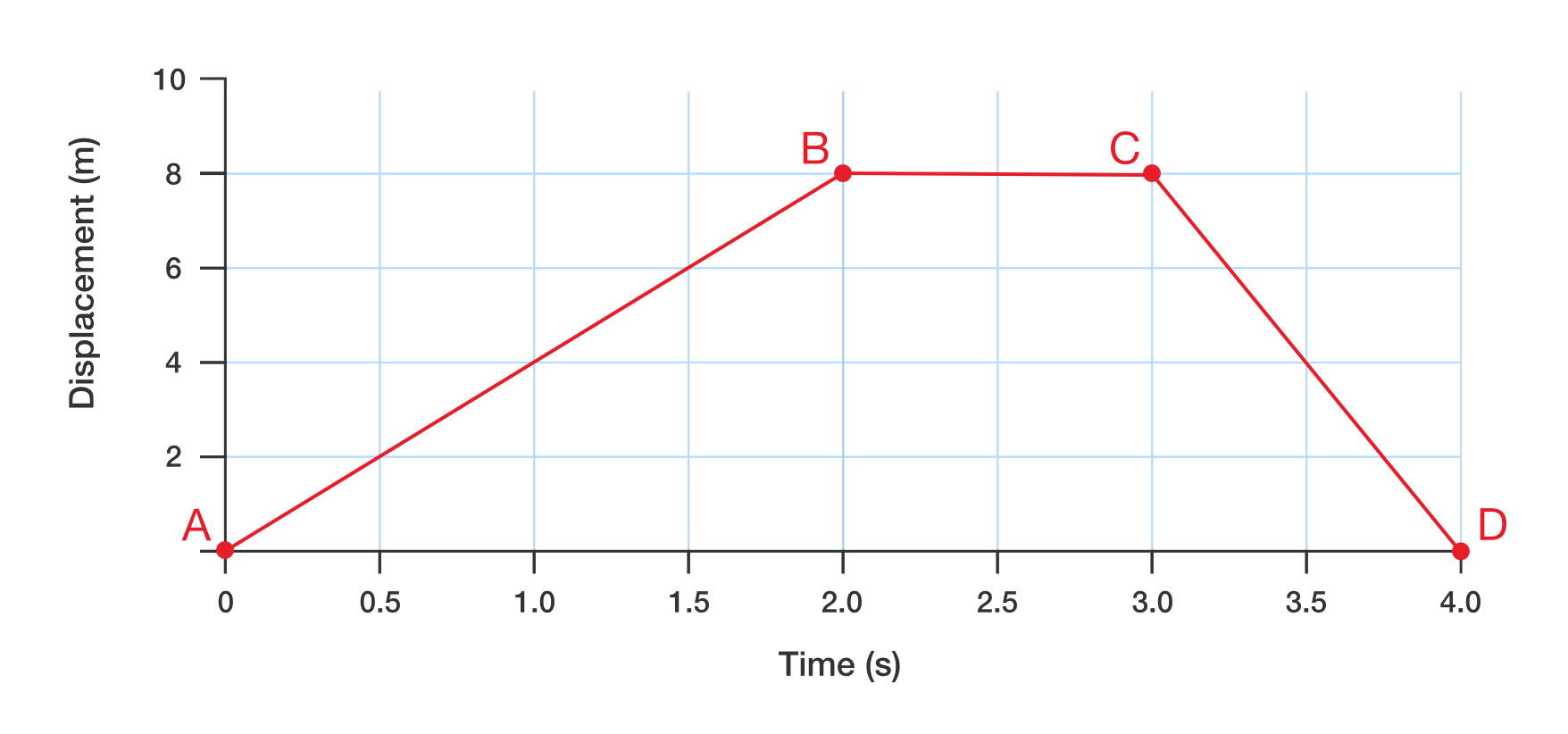
The gradient of a displacement (a vector quantity) versus time graph gives velocity (also a vector quantity). Expand the accordions to learn what is happening between each point on the graph.
From point A and B, the object is moving at constant velocity (the graph is a straight line). Its velocity \(v\) is the gradient of the line:
\[\begin{align*} v & = \frac{\text{displacement at B}-\text{displacement at A}}{\text{time at B}-\text{time at A}} \\[6pt]
& = \frac{8-0}{2-0}\\[6pt]
& = \frac{8}{2}\\[6pt]
& = 4\,\text{m/s}
\end{align*}\] This means that the object is moving at \(4\,\text{m/s}\).
From point B to C, the velocity is:
\[\begin{align*} v & = \frac{\text{displacement at C}-\text{displacement at B}}{\text{time at C}-\text{time at B}} \\[6pt]
& = \frac{8-8}{3-2}\\[6pt]
& = \frac{0}{1}\\[6pt]
& = 0\,\text{m/s}
\end{align*}\] There is no change in displacement as velocity is \(0\,\text{m/s}\).
From point C to D, the displacement decreases from \(8\text{ m}\) to \(0\text{ m}\) over a time of \(1\text{ s}\).
\[\begin{align*} v & = \frac{\text{displacement at D}-\text{displacement at C}}{\text{time at D}-\text{time at C}} \\[6pt]
& = \frac{0-8}{4-3}\\[6pt]
& = -\frac{8}{1}\\[6pt]
& = -8\text{ m/s}
\end{align*}\] The negative sign indicates that the object has reversed its direction and is moving at a speed of \(8\text{ m/s}\). At D, the object has returned to its starting position.
Velocity vs time graphs
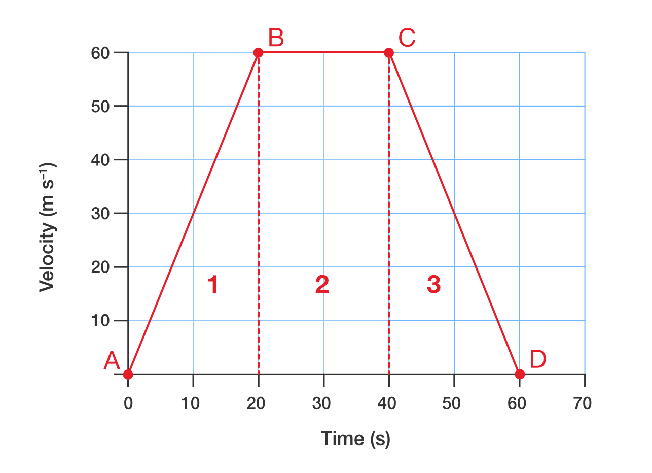
The velocity–time graph shows a car accelerating uniformly from rest to \(60\,\text{m/s}\) in \(20\,\text{s}\), then travels at a constant velocity of \(60\,\text{m/s}\) for the next \(20\,\text{s}\), then decelerates uniformly to rest in \(20\,\text{s}\). The total journey takes \(60\,\text{s}\).
From A to B, the object accelerates from \(0\,\text{m/s}\) to \(60\,\text{m/s}\). From B to C, the object moves at a constant velocity of \(60\,\text{m/s}\) and from C to D, the object slows to a stop from \(60\,\text{m/s}\).
Let's look at some features of the graph in detail: the area under the graph and its gradient.
Area under velocity–time graph
The area is the product of velocity and time, so the units are \(\text{m}/\text{s}\,\times \text{s}=\text{m}\). That is, the area under the graph gives displacement.
The area under a velocity–time graph gives displacement.
The area under a speed–time graph gives distance.
Consider the velocity–time graph again. The area has been divided into three regions: \(1\), \(2\) and \(3\). Let the area of each region be \(A_{1}\), \(A_{2}\) and \(A_{3}\), respectively. We have:
The gradient (or slope) of a velocity–time graph gives the acceleration of the object. It is calculated using:
\[m=\frac{\text{rise}}{\text{run}}\]
Expand the accordions to learn what is happening between each point on the graph.
From point A to B, the acceleration is:
\[\begin{align*} m_{AB} & = \frac{\text{rise}}{\text{run}} \\[6pt]
& = \frac{\text{change in velocity}}{\text{change in time}}\\[6pt]
& = \frac{60-0}{20-0}\\[6pt]
& = \frac{60}{20}\\[6pt]
& = 3\,\text{m}\,\text{s}^{-2}
\end{align*}\] The car is increasing its speed by \(3\,\text{m/s}\).
From point B to C, the acceleration is:
\[\begin{align*} m_{BC} & = \frac{\text{rise}}{\text{run}} \\[6pt]
& = \frac{\text{change in velocity}}{\text{change in time}}\\[6pt]
& = \frac{60-60}{40-20}\\[6pt]
& = \frac{0}{20}\\[6pt]
& = 0\,\text{m}\,\text{s}^{-2}
\end{align*}\] The car is not accelerating but is moving at a constant velocity of \(60\,\text{m/s}\).
From point C to D, the acceleration is:
\[\begin{align*} m_{CD} & =\frac{\text{rise}}{\text{run}} \\[6pt]
& = \frac{\text{change in velocity}}{\text{change in time}}\\[6pt]
& = \frac{0-60}{60-40}\\[6pt]
& = -\frac{60}{20}\\[6pt]
& = -3\,\text{m}\,\text{s}^{-2}\end{align*}\] The negative value of acceleration shows that the car is slowing down or decelerating.
What the gradient and area under each graph represents is summarised in the following table.
Graph type
Displacement–time
Velocity–time
Acceleration–time
Gradient
Velocity
Acceleration
No meaning
Area under graph
No meaning
Displacement
Change in velocity
Example 1 – sketching and describing linear motion graphs
A car accelerates from a stationary position. The rate of acceleration is constant. Sketch graphs of the acceleration versus time, the velocity versus time and the displacement versus time.
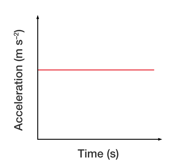
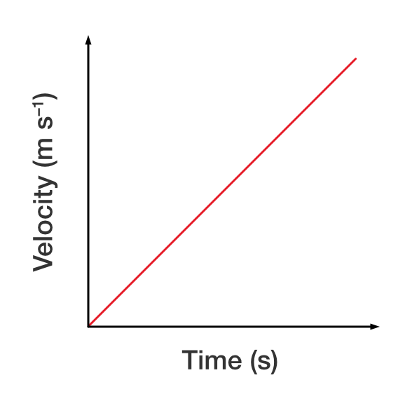
Since the acceleration is constant, the acceleration–time graph will simply be a horizontal line.
As the car is accelerating, this means that its velocity is increasing over time. The velocity–time graph is a linear graph with a gradient equal to acceleration.
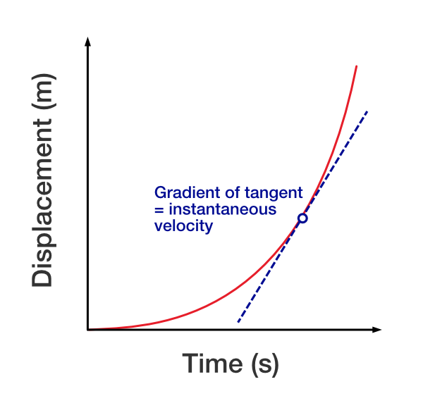
Displacement is the total distance travelled, so we get it by looking at how fast the car is going during each time interval. At the start, the car is moving slowly, so it does not cover much distance in the first few seconds. Later, it is moving faster, so it covers more distance in each second than before.
This means the displacement does not increase at a steady rate – it increases more and more quickly as time goes on, creating a curve.
The gradient (slope) at any point on the curve is the velocity at that time, or the instantaneous velocity. You can find the approximate value of the gradient by drawing a tangent at the point of interest and then calculating the gradient of the tangent.
A ball is thrown vertically upwards with a speed of \(\boldsymbol{5\,\textbf{m/s}}\). Sketch and describe the graph of velocity of the ball against time from the moment it is thrown to the moment it touches the ground. Ignore air resistance.
First, we need to define the coordinate system we want to work in. Let's take upwards velocity as positive and downwards velocity as negative. Once the ball is thrown up, the only force acting on it is gravity, which is constant. So from the previous example, the graph of velocity–time is linear.
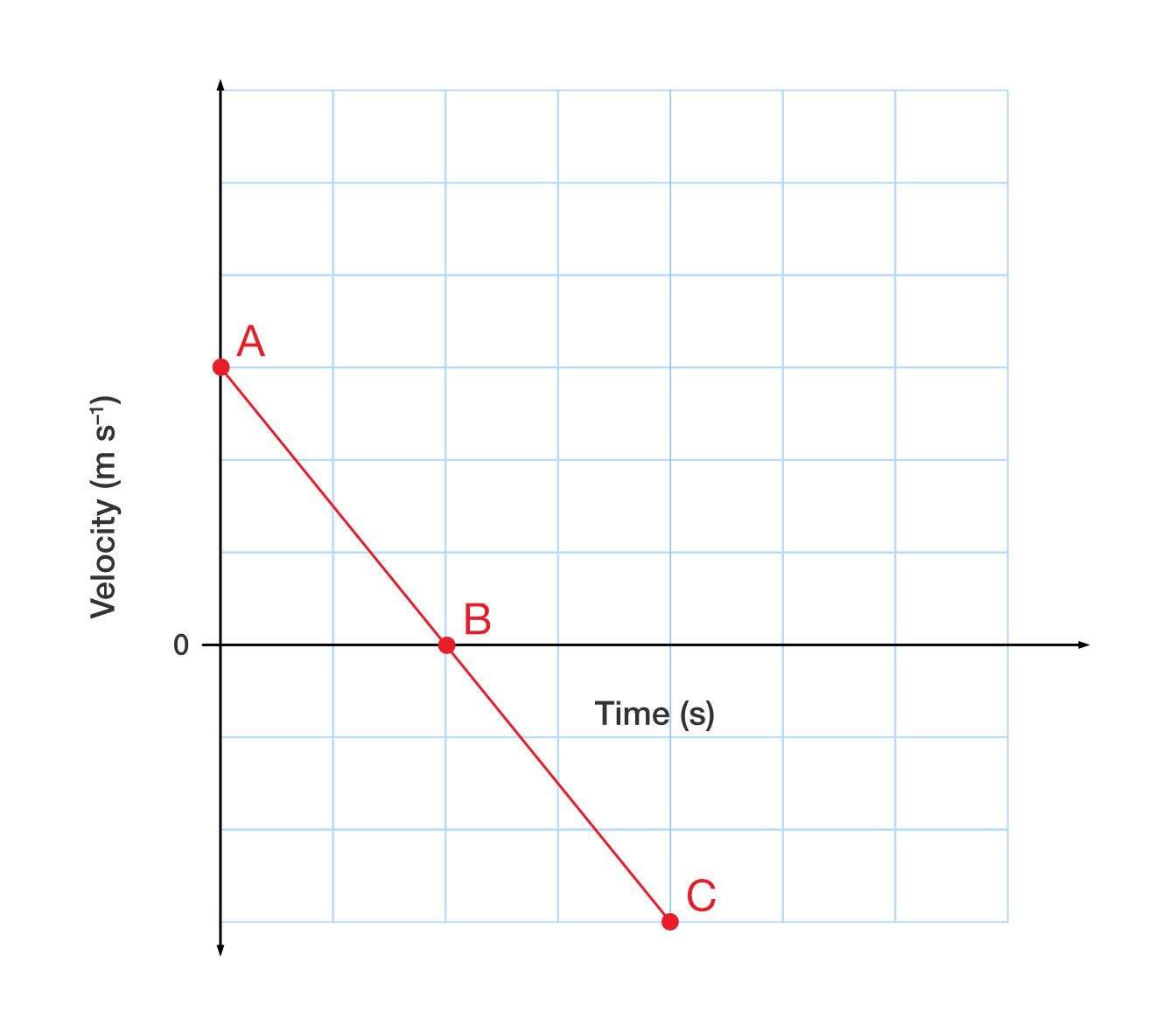
As gravity acts downwards, the velocity–time graph must have a negative gradient (because the ball is decelerating). This gives us the following velocity–time graph:
To describe it, let's think about what has happened: Initially the ball is thrown into the air vertically upwards (positive direction) with a speed of \(5\,\text{m/s}\). Point A describes the initial upward velocity that the ball has. It is \(5\,\text{m/s}\) upward.
Then, the ball starts to slow down due to gravity acting on it. This is the part of the graph from A to B. At point B, the ball is not moving. This is the point of maximum altitude for the ball where it has zero velocity.
After B, the ball is now heading downwards towards the point from which it was thrown (point C). It has a negative velocity of \(-5\,\text{m/s}\), or \(5\,\text{m/s}\) downward. At point C, the ball has the same speed as it had at point A.
Exercise – sketching and describing linear motion graphs
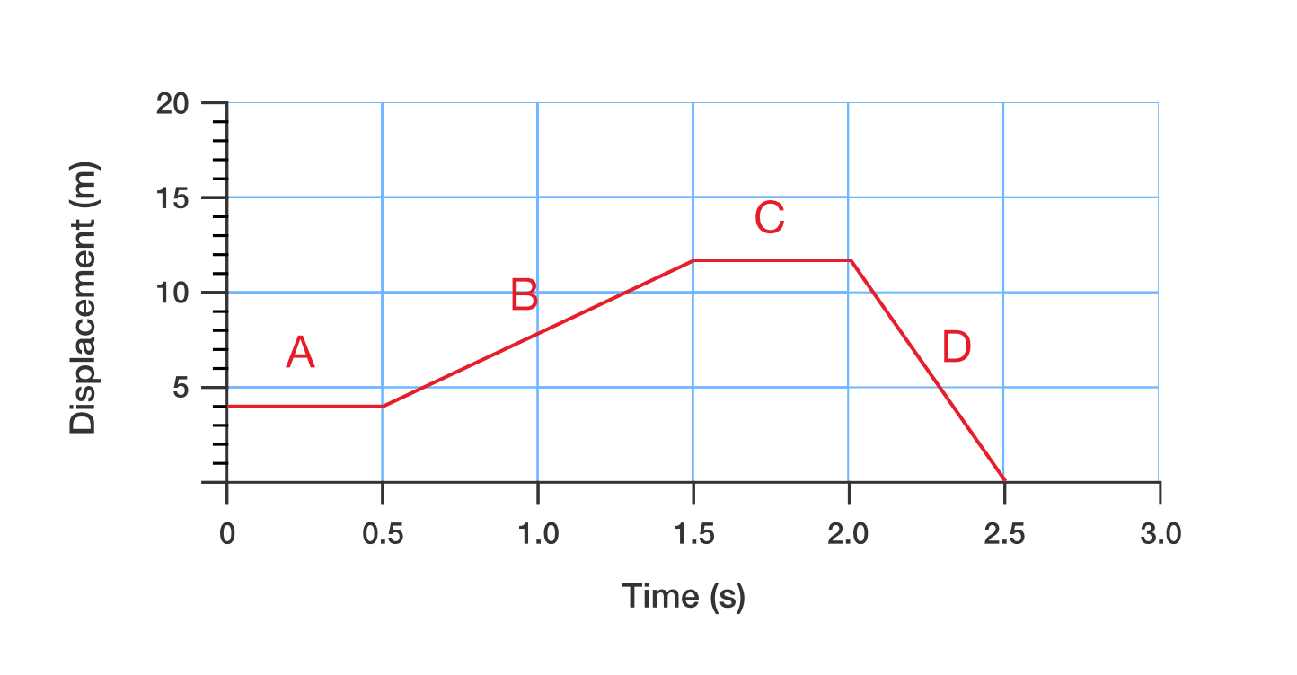
The graph shows the position (displacement) of a dancer moving in a straight line across a stage. The dancer’s movements are designated by sections A to D.
Determine the dancer's starting position.
Determine in which section (A—D) the dancer is at rest.
Determine in which section the dancer is moving in a positive direction.
Determine in which sections the dancer is moving with a negative velocity.
\(+4\,\text{m}\)
Sections A and C
Section B
Section D
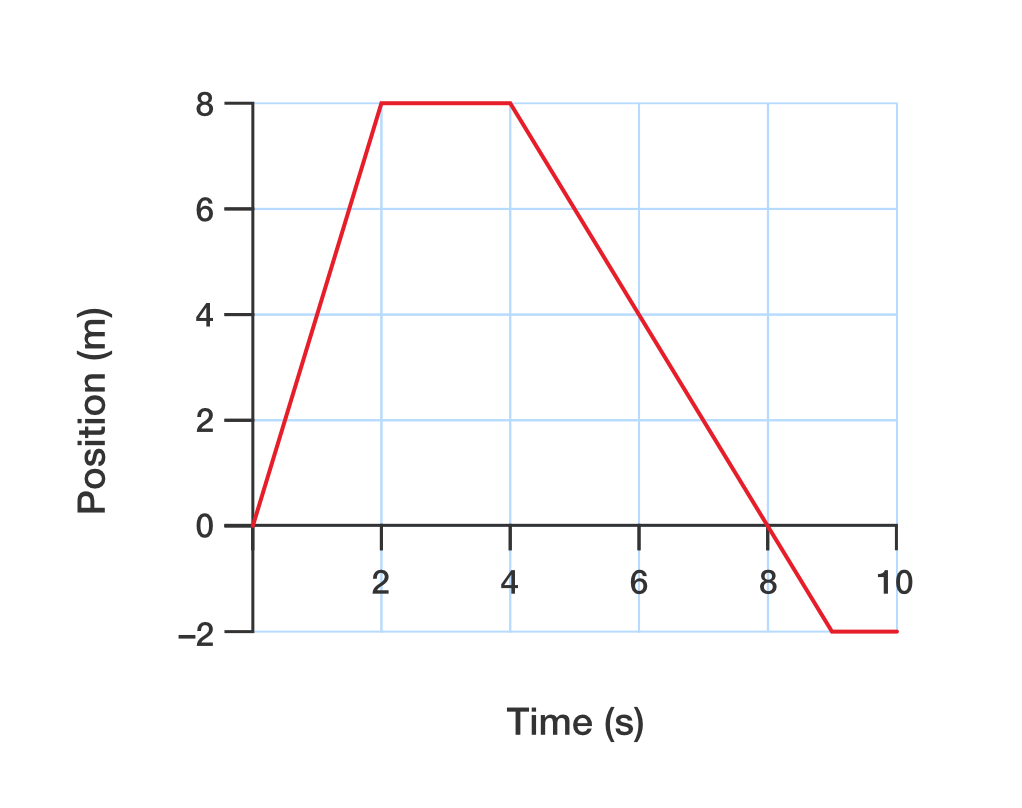
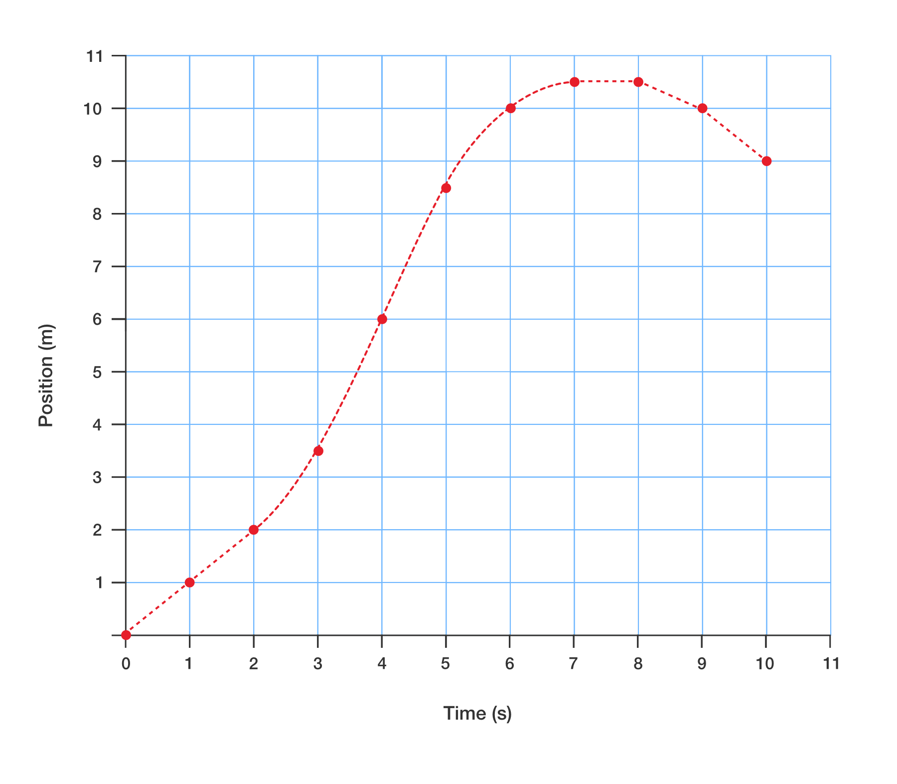
The graph represents the straight line motion of a radio-controlled toy car.
Describe, in words, the motion of the car.
Determine the position of the car at:
\(2\,\text{s}\)
\(4\,\text{s}\)
\(6\,\text{s}\)
\(10\,\text{s}\).
Determine at what time the car returned to its starting point.
Calculate the velocity of the car:
during the first \(2\,\text{s}\)
at \(3\,\text{s}\)
from \(4\,\text{s}\) to \(6\,\text{s}\)
at \(8\,\text{s}\)
from \(8\,\text{s}\) to \(9\,\text{s}\).
During its \(10\,\text{s}\) motion, calculate the car's:
distance travelled
displacement.
The car initially moves in a positive direction and travels \(8\,\text{m}\) in \(2\,\text{s}\). It then stops for \(2\,\text{s}\). The car then reverses direction for \(5\,\text{s}\), passing back through its starting point at \(8\,\text{s}\). It then travels a further \(2\,\text{m}\) in a negative direction before stopping after \(9\,\text{s}\).
\(+8\,\text{m}\)
\(+8\,\text{m}\)
\(+4\,\text{m}\)
\(-2\,\text{m}\)
\(8\,\text{s}\)
\(+4\,\text{m/s}\)
\(0\,\text{m/s}\)
\(-2\,\text{m/s}\)
\(-2\,\text{m/s}\)
\(-2\,\text{m/s}\)
\(18\,\text{m}\)
\(-2\,\text{m}\)
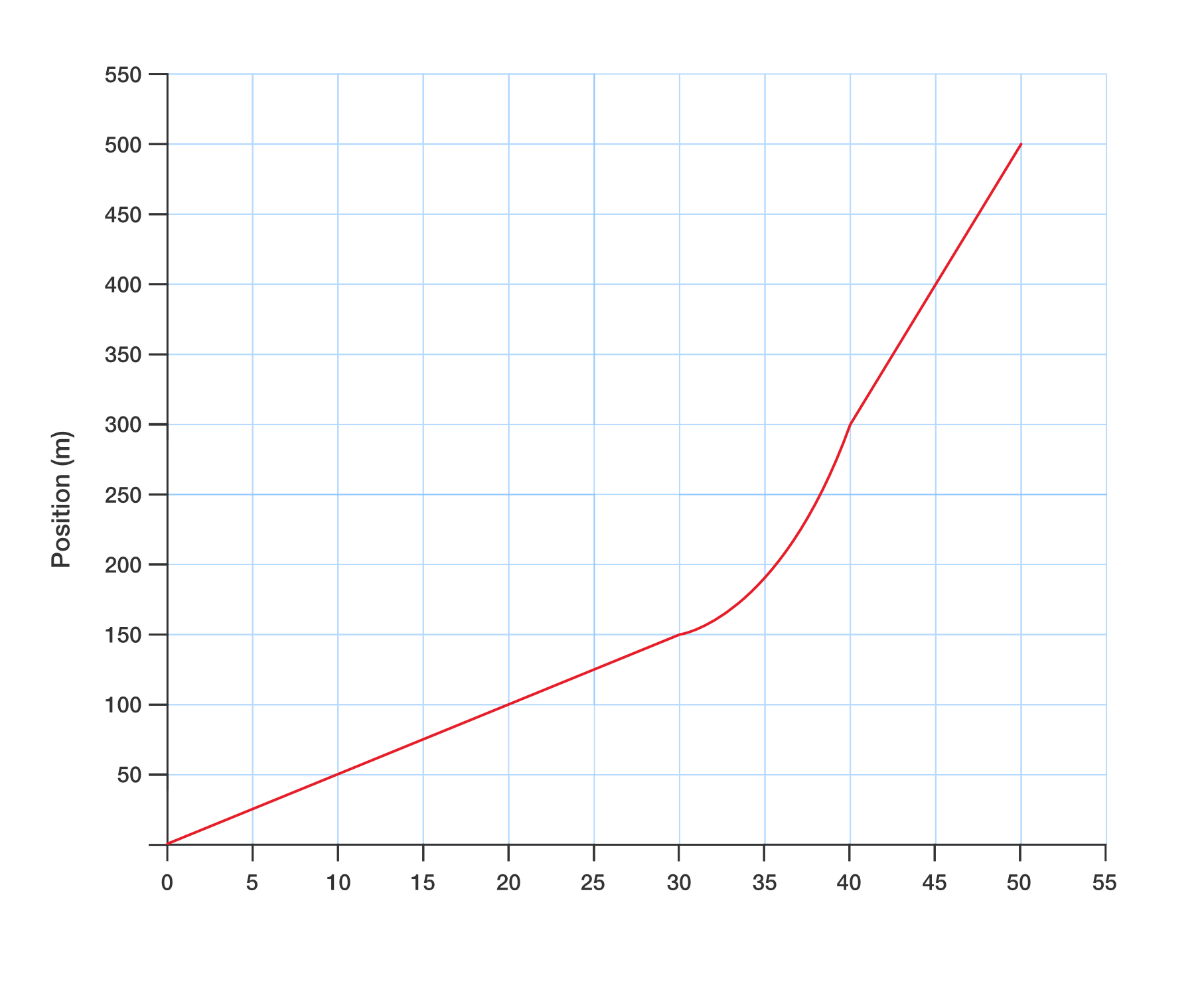
The following position–time graph is for a cyclist travelling along a straight road.
Describe, in words, the motion of the cyclist.
Calculate the velocity of the cyclist during the first \(30\,\text{s}\).
Calculate the cyclist’s velocity during the final \(10\,\text{s}\).
Estimate the cyclist’s instantaneous velocity at \(35\,\text{s}\).
Determine the average velocity of the cyclist between \(30\,\text{s}\) and \(40\,\text{s}\).
The cyclist travels with a constant velocity in a positive direction for the first \(30\,\text{s}\) and travels \(150\,\text{m}\) in this time. Then, the cyclist speeds up for the next \(10\,\text{s}\), travelling a further \(150\,\text{m}\). Finally, the cyclist maintains the increased speed for the final \(10\,\text{s}\) and covers another \(200\,\text{m}\) in this time.
\(+5\,\text{m/s}\)
\(+20\,\text{m/s}\)
\(13\,\text{m/s}\)
\(+15\,\text{m/s}\)
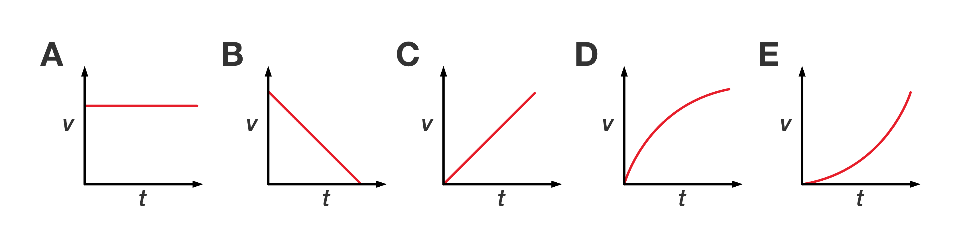
Consider the velocity–time graphs, A to E.
Identify which velocity-time graph best represents the motion of:
a car coming to a stop at a traffic light
a swimmer moving at a constant speed
a cyclist accelerating from rest with constant acceleration
a car accelerating from rest and changing through its gears.
Graph B
Graph A
Graph C
Graph D.
Note: Graph D shows the car's speed increasing but by smaller amounts each second (matching an engine that loses pulling power as it gears up and speeds up), while graph E shows speed increasing by larger amounts each second, which no real engine can do.
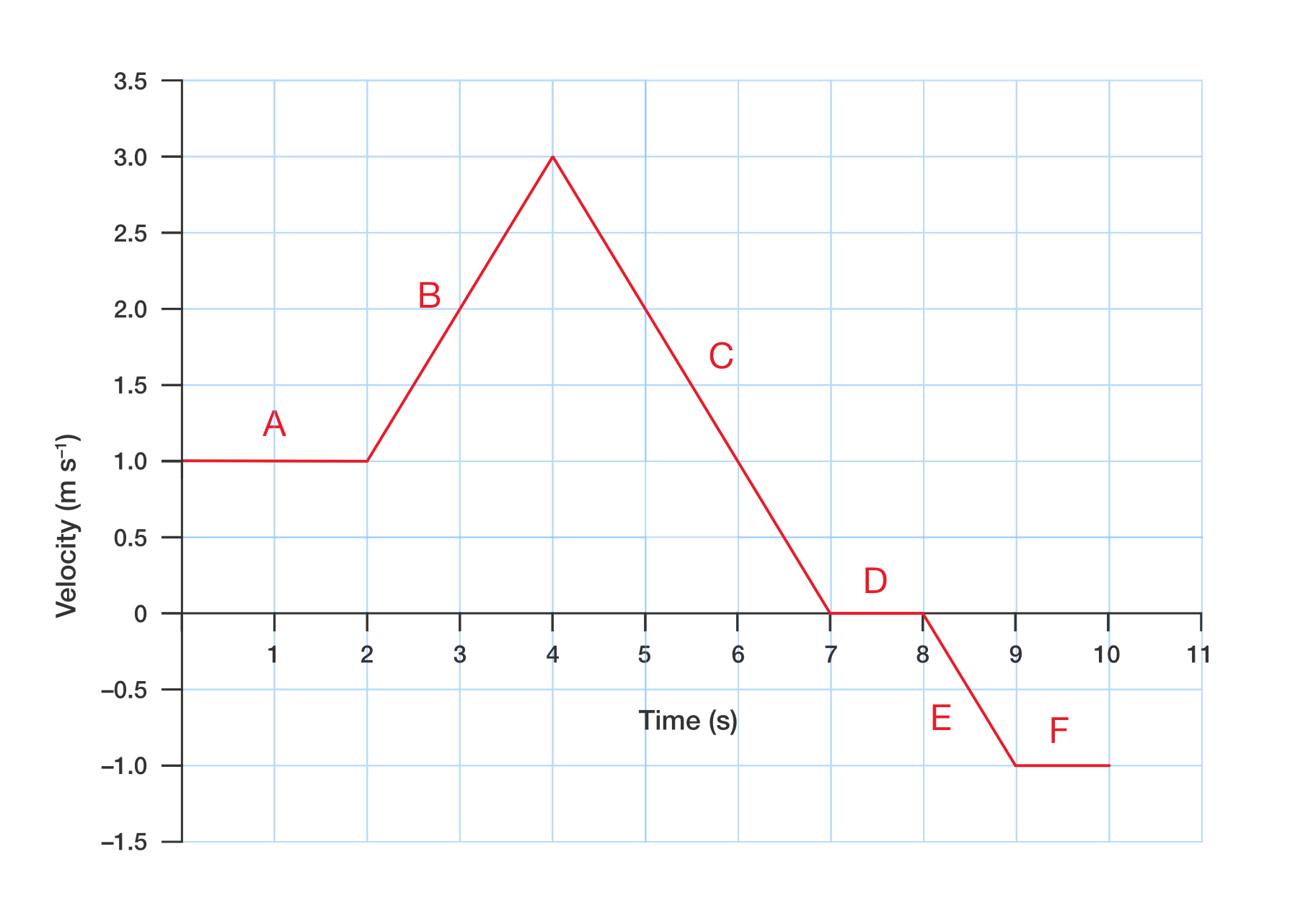
The following graph shows the motion of a dog running along a footpath in a northerly direction.
Describe the motion of the dog during each section of the graph (A to F).
Calculate the displacement of the dog after:
\(2\,\text{s}\)
\(7\,\text{s}\)
\(10\,\text{s}\)
Plot a position–time graph for the dog’s motion.
The dog runs North at \(1\,\text{m/s}\) during section A, then increases to \(3\,\text{m/s}\) while running North during section B. In section C, it is slowing to a stop and becomes stationary at section D. During section E, the dog accelerates from rest to \(1\,\text{m/s}\) while travelling South. It continues running South at \(1\,\text{m/s}\) during section F.
\(2\,\text{m}\)
\(10.5\,\text{m}\)
\(9\,\text{m}\)
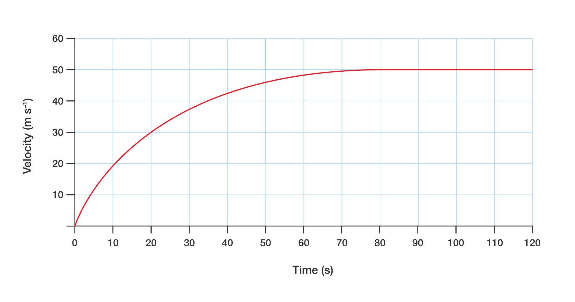
The straight line motion of a train is shown in the following velocity–time graph.
Determine how long the train takes to reach its cruising speed.
Calculate the acceleration of the train \(10\,\text{s}\) after starting. (Hint: You can only approximate this. Take a tangent to the graph at \(10\,\text{s}\) and calculate its gradient.)
Calculate the acceleration of the train \(40\,\text{s}\) after starting
Calculate the approximate displacement of the train after \(120\,\text{s}\).
\(80\,\text{s}\)
\(2\,\text{m/s}^{2}\)
\(0.2\,\text{m/s}^{2}\)
\(4800\,\text{m}\)
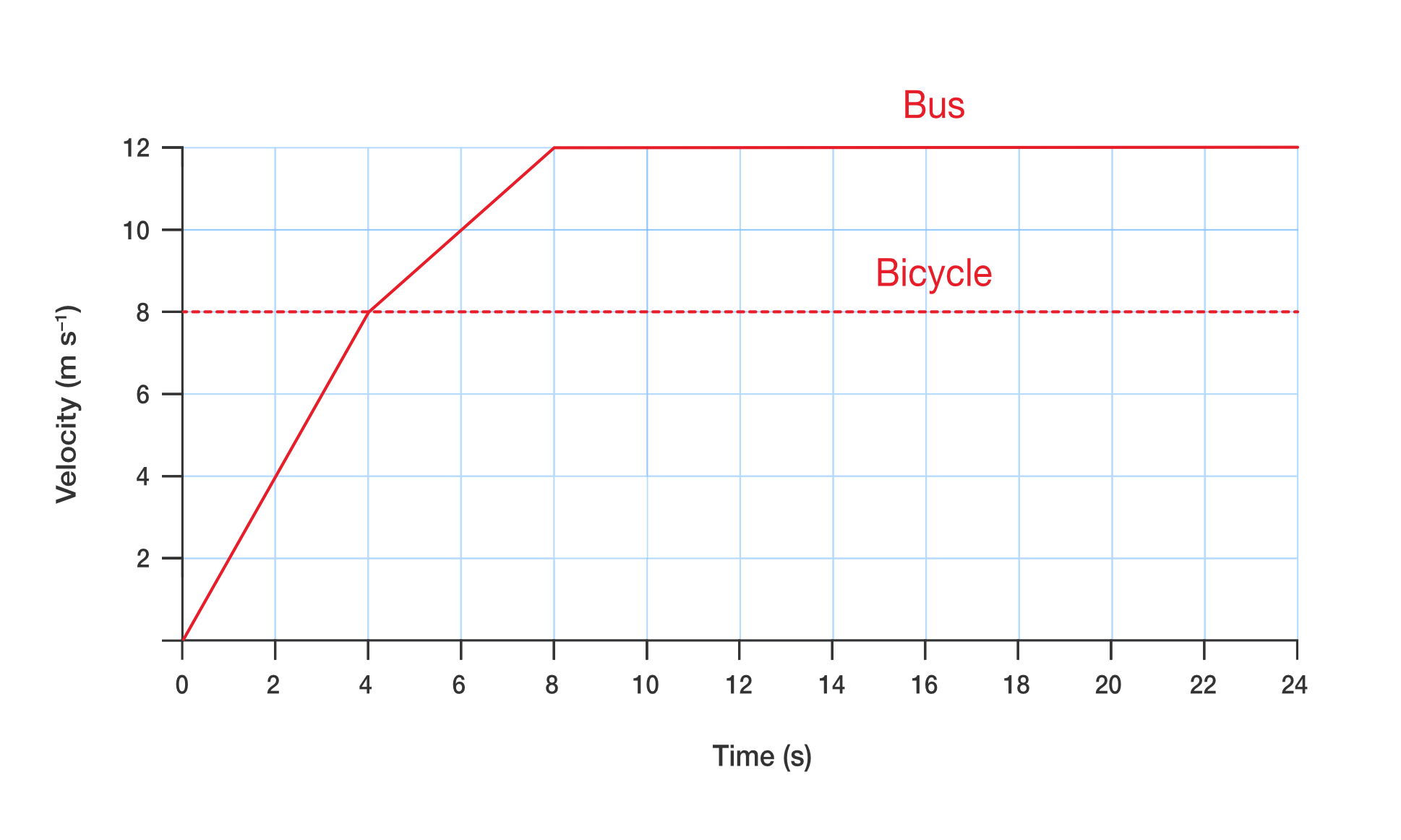
The velocity–time graphs for a bus and a bicycle travelling along the same straight stretch of road are shown in the graph. The bus is initially at rest and starts moving as the bicycle passes it.
Calculate the initial acceleration of the bus.
Determine at what time the bus first starts gaining ground on the bicycle.
Determine at what time the bus overtakes the bicycle.
Determine how far the bicycle has traveled before the bus catches up to it.
Determine the average velocity of the bus during the first \(8\,\text{s}\).
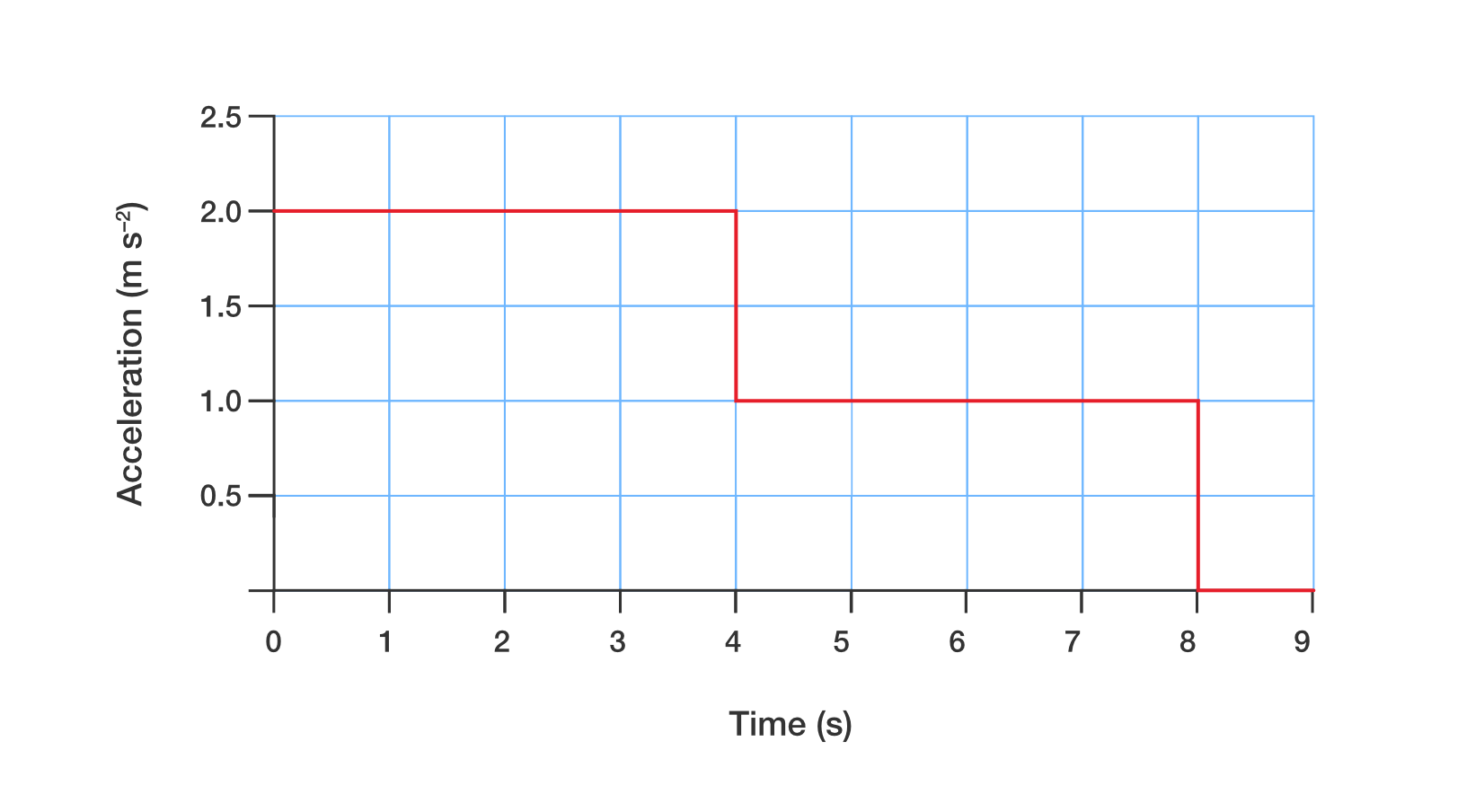
Draw an acceleration–time graph for the bus.
Use your acceleration–time graph to determine the change in velocity of the bus over the first \(8\,\text{s}\).
\(+2\,\text{m/s}\)
\(4\,\text{s}\) – this is when the two lines intersect
\(10\,\text{s}\) – this is when the bus and bicycle have covered the same distance, i.e. area under the curve is the same