A standard normal distribution helps us compare different datasets by converting them to a common scale using values called \(z\)-scores. Understanding standard normal distributions makes it easier to calculate probabilities and assess how individual data points relate to the average. Use this resource to learn how to analyse standard normal distributions and use \(z\)-tables.
\(z\)-distributions
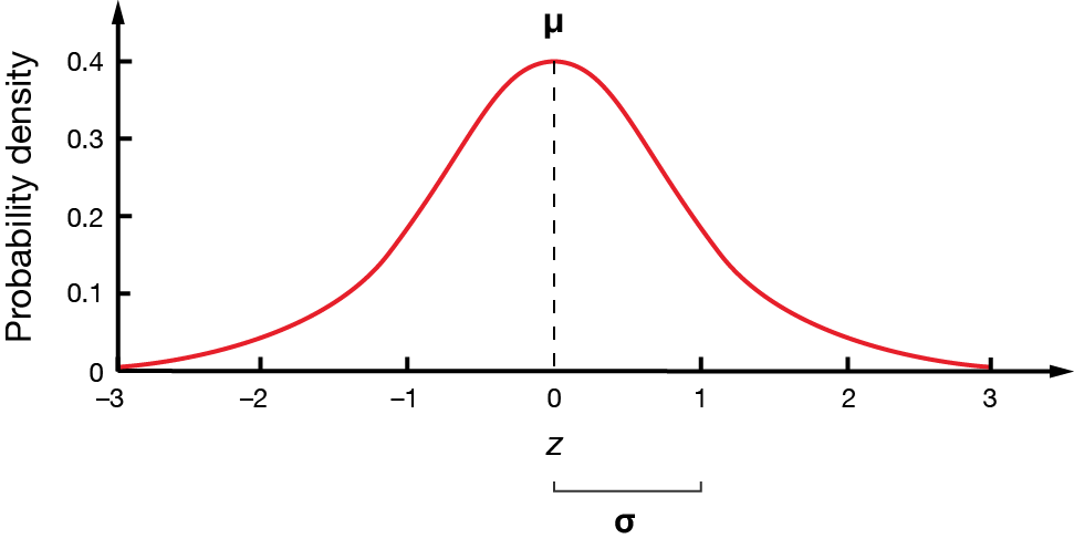
A normal distribution with a mean of \(\mu=0\) and a standard deviation of \(\sigma=1\) is called the standard normal distribution.
\(z\)-tables
Areas under the standard normal distribution curve represent probabilities which can be found using a calculator or a \(z\)-table.
The \(z\)-score represents how many standard deviations a data point is from the mean in a standard normal distribution. For example, if \(z=0.05\), then the data point is \(0.05\) standard deviations above the mean. Typical \(z\)-tables only show positive standard deviations, but since the standard normal distribution is symmetrical, we can still find the answers we are looking for.
When we work with the standard normal distribution, we are not restricted to \(1\), \(2\) and \(3\) standard deviations from the mean and the \(68-95-99\) rule for other normal distributions. \(z\)-tables let us find proportions, percentages or probabilities for any value in the distribution.
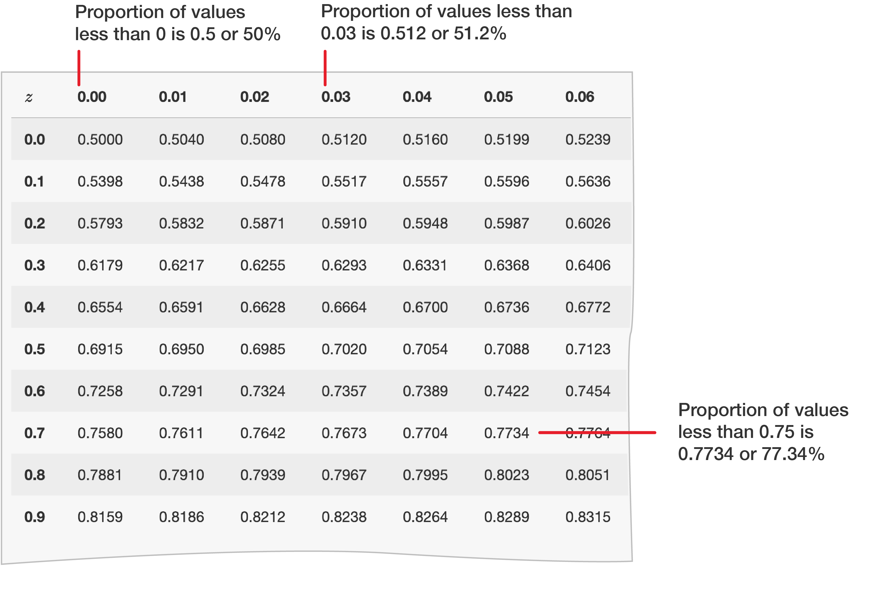
\(z\)-tables come in different layouts, but here, we show a small section of a table that gives \(z\)-values up to \(2\) decimal places.
Interpreting \(z\)-tables
When using a \(z\)-table, you need to look at your \(z\)-score in two parts. Let's consider \(z=1.32\). You would need to break this up into:
\[1.30+0.02\]
The larger value, \(1.30\), is found in the first column of the table. The smaller value \(0.02\) is found in the first row. The corresponding area value in the table is the proportion, percentage or probability that \(z\) is less than \(1.32\).
Some other examples are:
\(\Pr(z<0.00)=0.500\) or \(50\%\). This is \(0.0\) in the first column and \(0.00\) in the first row.
\(\Pr(z<0.03)=0.512\) or \(51.2\%\). This is \(0.0\) in the first column and \(0.03\) in the first row.
\(\Pr(z<0.75)=0.7734\) or \(77.34\). This is \(0.7\) in the first column and \(0.05\) in the first row.
You can also use a graphics calculator or computer (instead of a \(z\)-table) to find areas, proportions and probabilities in a normal distribution.
Example 1 – interpreting \(z\)-tables
In a standard normal distribution, what percentage of values will be less than \(1.28\)?
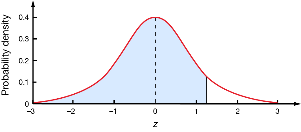
It is always good to start with a diagram of the standard normal distribution. It will also help you sense-check your answer.
From this, it is clear that we are looking for the shaded area to the left of \(z=1.28\). We can use the following table to find that the area to the left is \(0.8997\).]
Standard normal distribution: table values represent area to the left of the Z score.
\(z\)
.00
.01
.02
.03
.04
.05
.06
.07
.08
.09
0.0
0.50000
0.50399
0.50798
0.51197
0.51595
0.51994
0.52392
0.52790
0.53188
0.53586
0.1
0.53983
0.54380
0.54776
0.55172
0.55567
0.55962
0.56356
0.56749
0.57142
0.57535
0.2
0.57926
0.58317
0.58706
0.59095
0.59483
0.59871
0.60257
0.60642
0.61026
0.61409
0.3
0.61791
0.62171
0.62552
0.62930
0.63307
0.63683
0.64058
0.64431
0.64803
0.65173
0.4
0.65542
0.65910
0.66276
0.66640
0.67003
0.67364
0.67724
0.68082
0.68439
0.68793
0.5
0.69146
0.69497
0.69847
0.70194
0.70540
0.70884
0.71226
0.71566
0.71904
0.72240
0.6
0.72575
0.72907
0.73237
0.73565
0.73891
0.74215
0.74537
0.74857
0.75175
0.75490
0.7
0.75804
0.76115
0.76424
0.76730
0.77035
0.77337
0.77637
0.77935
0.78230
0.78524
0.8
0.78814
0.79103
0.79389
0.79673
0.79955
0.80234
0.80511
0.80785
0.81057
0.81327
0.9
0.81594
0.81859
0.82121
0.82381
0.82639
0.82894
0.83147
0.83398
0.83646
0.83891
1.0
0.84134
0.84375
0.84614
0.84849
0.85083
0.85314
0.85543
0.85769
0.85993
0.86214
1.1
0.86433
0.86650
0.86864
0.87076
0.87286
0.87493
0.87698
0.87900
0.88099
0.88296
1.2
0.88493
0.88686
0.88877
0.89065
0.89251
0.89435
0.89617
0.89796
0.89973
0.90147
1.3
0.90320
0.90490
0.90658
0.90824
0.90988
0.91149
0.91309
0.91466
0.91621
0.91774
1.4
0.91924
0.92073
0.92220
0.92364
0.92507
0.92647
0.92785
0.92922
0.93056
0.93189
1.5
0.93319
0.93448
0.93574
0.93699
0.93822
0.93943
0.94062
0.94179
0.94295
0.94408
This means that \(89.97\%\) of values will be less than \(1.28\). This agrees with the shaded region in our diagram; a large proportion of the curve is shaded.
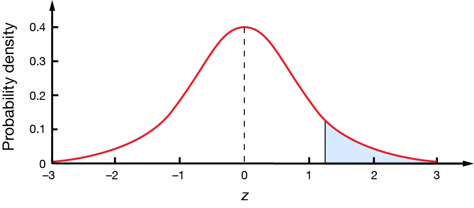
In a standard normal distribution, what percentage of values will be more than \(1.28\)?
Again, let's make a diagram. We want to find the percentage area shown.
We cannot use the \(z\)-tables on this page to find areas to the right of a \(z\)-score. Instead, we can find the unshaded area and minus it from \(100\%\).
Here, we know that \(89.97\%\) of the values are less than \(1.28\), so \(100-89.97=10.03\%\) of values will be more than \(1.28\).
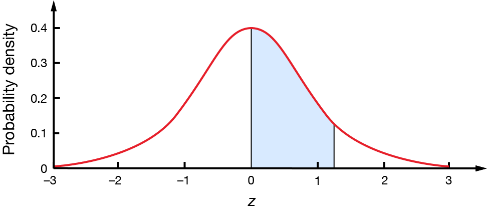
In a standard normal distribution, what percentage of values will be between \(0\) and \(1.28\)?
We want to find the percentage area shown.
We cannot look up areas between two values directly from the table but we know that \(89.97\%\) of values are less than \(1.28\). We also know that \(50\%\) of values lie to the left of the mean \((z=0)\) because the bell curve is symmetrical.
Therefore, the percentage of values between \(0\) and \(1.28\) is \(89.97-50=39.97\%\).
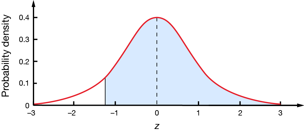
In a standard normal distribution, what percentage of values will be greater than \(-1.28\)?
We want to find the percentage area shown.
Although there are some normal distribution tables that include negative \(z\)-scores, we cannot usually look up negative values in a \(z\)-table. We do know that the bell curve is symmetrical, so the area to the right of \(-1.28\) is the same as the area to the left of \(1.28\).
Therefore, the percentage of values greater than \(-1.28\) is \(89.97\%\).
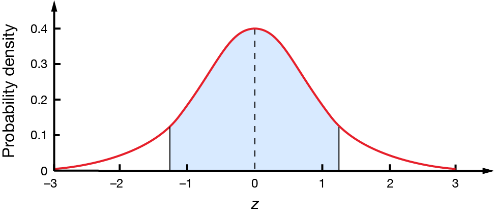
In a standard normal distribution, what percentage of values will be between \(-1.28\) and \(1.28\)?
To find this area, we use the symmetry of the distribution. We can see that the area between \(-1.28\) and \(0\) is exactly the same as the area between \(0\) and \(1.28\).
We know the area between \(0\) and \(1.28\) is \(39.97\%\). Therefore, the percentage of the graph between \(-1.28\) and \(1.28\) is \(2\times39.97=79.8\%\).
Exercise – interpreting \(z\)-tables
Use the following \(z\)-table to answer the questions.
\(z\)
0.00
0.01
0.02
0.03
0.04
0.05
0.06
0.07
0.08
0.09
0.0
0.5000
0.5040
0.5080
0.5120
0.5160
0.5199
0.5239
0.5279
0.5319
0.5359
0.1
0.5398
0.5438
0.5478
0.5517
0.5557
0.5596
0.5636
0.5675
0.5714
0.5753
0.2
0.5793
0.5832
0.5871
0.5910
0.5948
0.5987
0.6026
0.6064
0.6103
0.6141
0.3
0.6179
0.6217
0.6255
0.6293
0.6331
0.6368
0.6406
0.6443
0.6480
0.6517
0.4
0.6554
0.6591
0.6628
0.6664
0.6700
0.6736
0.6772
0.6808
0.6844
0.6879
0.5
0.6915
0.6950
0.6985
0.7019
0.7054
0.7088
0.7123
0.7157
0.7190
0.7224
0.6
0.7257
0.7291
0.7324
0.7357
0.7389
0.7422
0.7454
0.7486
0.7517
0.7549
0.7
0.7580
0.7611
0.7642
0.7673
0.7704
0.7734
0.7764
0.7794
0.7823
0.7852
0.8
0.7881
0.7910
0.7939
0.7967
0.7995
0.8023
0.8051
0.8078
0.8106
0.8133
0.9
0.8159
0.8186
0.8212
0.8238
0.8264
0.8289
0.8315
0.8340
0.8365
0.8389
1.0
0.8413
0.8438
0.8461
0.8485
0.8508
0.8531
0.8554
0.8577
0.8599
0.8621
1.1
0.8643
0.8665
0.8686
0.8708
0.8729
0.8749
0.8770
0.8790
0.8810
0.8830
1.2
0.8849
0.8869
0.8888
0.8907
0.8925
0.8944
0.8962
0.8980
0.8997
0.9015
1.3
0.9032
0.9049
0.9066
0.9082
0.9099
0.9115
0.9131
0.9147
0.9162
0.9177
1.4
0.9192
0.9207
0.9222
0.9236
0.9251
0.9265
0.9279
0.9292
0.9306
0.9319
1.5
0.9332
0.9345
0.9357
0.9370
0.9382
0.9394
0.9406
0.9418
0.9429
0.9441
1.6
0.9452
0.9463
0.9474
0.9484
0.9495
0.9505
0.9515
0.9525
0.9535
0.9545
1.7
0.9554
0.9564
0.9573
0.9582
0.9591
0.9599
0.9608
0.9616
0.9625
0.9633
1.8
0.9641
0.9649
0.9656
0.9664
0.9671
0.9678
0.9686
0.9693
0.9699
0.9706
1.9
0.9713
0.9719
0.9726
0.9732
0.9738
0.9744
0.9750
0.9756
0.9761
0.9767
2.0
0.9772
0.9778
0.9783
0.9788
0.9793
0.9798
0.9803
0.9808
0.9812
0.9817
2.1
0.9821
0.9826
0.9830
0.9834
0.9838
0.9842
0.9846
0.9850
0.9854
0.9857
2.2
0.9861
0.9864
0.9868
0.9871
0.9875
0.9878
0.9881
0.9884
0.9887
0.9890
2.3
0.9893
0.9896
0.9898
0.9901
0.9904
0.9906
0.9909
0.9911
0.9913
0.9916
2.4
0.9918
0.9920
0.9922
0.9925
0.9927
0.9929
0.9931
0.9932
0.9934
0.9936
2.5
0.9938
0.9940
0.9941
0.9943
0.9945
0.9946
0.9948
0.9949
0.9951
0.9952
2.6
0.9953
0.9955
0.9956
0.9957
0.9959
0.9960
0.9961
0.9962
0.9963
0.9964
2.7
0.9965
0.9966
0.9967
0.9968
0.9969
0.9970
0.9971
0.9972
0.9973
0.9974
2.8
0.9974
0.9975
0.9976
0.9977
0.9977
0.9978
0.9979
0.9979
0.9980
0.9981
2.9
0.9981
0.9982
0.9982
0.9983
0.9984
0.9984
0.9985
0.9985
0.9986
0.9986
In a standard normal distribution, what percentage of values will be:
less than \(1.95\)?
less than \(-1.95\)?
between \(-1.95\) and \(0\)?
greater than \(1.95\)?
between \(-1.95\) and \(1.95\)?
In a standard normal distribution, what proportion of values lie between \(-0.5\) and \(1.5\)?
In a standard normal distribution, what proportion of values lie outside the interval \(\pm1.7\)?
Given that a value in a standard normal distribution is greater than \(-1\), what is the probability that it will be less than \(2\)? (Hint: use the conditional probability formula.)
\(97.44\%\)
\(2.56\%\)
\(47.44\%\)
\(2.56\%\)
\(94.88\%\)
\(0.6247\)
\(0.0892\)
\(0.9729\)
Standard normal distributions in context
In accounting, a firm processes a large number of tax returns, and the time it takes to complete a return is normally distributed. The firm's management has determined that the standardised time (\(z\)-score) for completing a standard tax return is used to measure efficiency.
The firm's efficiency target is to complete a tax return with a \(z\)-score between \(-1.5\) and \(1.5\). Using the standard normal distribution, what percentage of tax returns fall within this target range?
The area under the curve for \(z\)-values less than \(1.5\) is \(0.9332\). The area under the curve for \(z\)-values less than \(0\) is \(0.5000\), so this means the area under the curve between \(0\) and \(1.5\) is \(0.9332-0.5000=0.4332\) or \(43.32\%\).
Since the curve is symmetrical, the area under the curve will be the same between \(-1.5\) and \(0\). Therefore, \(2\times43.32=86.64\%\) of the tax returns fall within this target range.