Working out a marketing budget
Explore these skills in a real world context.
The mean, mode, and median provide a single value that is typical of the data. These measures of central tendency help summarise large datasets, making it easier to understand the overall pattern. Understanding these concepts is essential for analysing and interpreting data effectively.
The mean, median, and mode are important tools for understanding data. They each give a single value that represents the data as a whole. These are called measures of central tendency because they show the centre or most typical values in a dataset, helping us quickly see what is common or typical.
where \(n\) is the total number of data points. If the value is \(4\), the median will be the fourth value in the ordered dataset.
where \(\sum x_{n}\) is the sum of each score \(x\) multiplied by its frequency (f).
Consider the data set \(3,2,0,5,2\). Find the mode, median and mean.
To find the mode, we find the value that occurs most frequently in the dataset. The mode is \(2\) because it occurs twice.
To find the median, we need to rearrange the data so that it is ordered from smallest to largest and find the middle number:
\[0,2,\underline{2},3,5\]
The median is \(2\).
To find the mean, we use \(\overline{x}=\dfrac{\sum x_{i}}{n}\).
\[\begin{align*} \overline{x} & = \frac{\sum x_{i}}{n}\\
& = \frac{3+2+0+5+2}{5}\\
& = 2.4
\end{align*}\]
The mean is \(2.4\).
| \(x\) | Frequency (f) |
|---|---|
| \(-3\) | \(1\) |
| \(-1\) | \(3\) |
| \(4\) | \(1\) |
| \(5\) | \(2\) |
| \(24\) | \(1\) |
The mode is \(-1\), which occurs \(3\) times.
When we reorder the frequencies from smallest to largest, there are \(8\) values, meaning that there are two ‘middle’ values.
\[-3,-1,-1,\underbrace{-1,4}_{\text{Middle scores}},5,5,24\]
The median is the average of these two middle values:
\[\begin{align*} \text{Median} & = \frac{-1+4}{2}\\
& = 1.5
\end{align*}\]
The mean is:
\[\frac{(-3\times1(+(-1\times3)+(4\times1)+(5\times2)+(24\times1)}{8}=4\]
Note that a disadvantage of the mean is that it is affected or distorted by extreme or outlying values.
| Score | Frequency |
|---|---|
| \(40\) | \(1\) |
| \(50\) | \(4\) |
| \(60\) | \(8\) |
| \(70\) | \(3\) |
| \(80\) | \(3\) |
| \(90\) | \(1\) |
The mode is the value that appears most frequently. All the sales figures are unique, so there is no mode.
The median is the middle value when the sales figures are ordered.
\[450,500,\underline{475},490,530\]
We can visualise measures of central tendency using bell curves and stem-and-leaf plots. These tools make it easier to interpret data and understand its key characteristics.
A bell curve or normal distribution graphically shows the mean in the centre with data symmetrically distributed around it. This shape highlights how values are spread out, with most clustering around the mean.
Consider this example. It is a symmetrical, bell-shaped distribution graph, where the mode, median and mean all have the same value, \(100\).
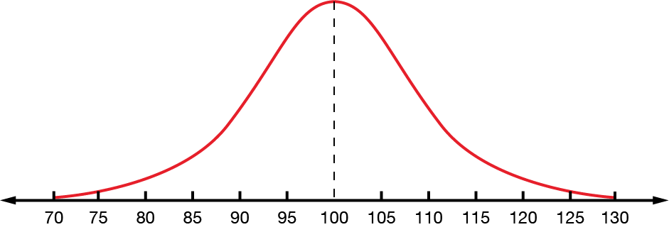
Learn more about normal distributions on this page.
Stem and leaf plots organise data to display the shape and distribution. They let us quickly see the median and mode, as well as the overall spread of the data.
Consider the following dataset.
\[1,1,,2,7,11,13,13,14,18,20,22,\ldots,86,94,96\]
We can organise this data in a stem and leaf plot.
\[\begin{array}{ccccccccccc} & 0 & \mid & & 1 & 1 & 2 & 7\\
& 1 & \mid & & 1 & 3 & 3 & 4 & 8\\
& 2 & \mid & & 0 & 2 & 3 & 7 & 9\\
& 3 & \mid & & 2 & 3 & 4 & 5 & 5 & 5 & 8\\
& 4 & \mid & & 1 & 4 & 7 & 8 & 8 & 9 & 9\\
& 5 & \mid & & 0 & 2 & 4 & 5 & 7 & 8\\
& 6 & \mid & & 1 & 4 & 5 & 6 & 9\\
& 7 & \mid & & 4 & 7 & 8\\
& 8 & \mid & & 0 & 2 & 5 & 6\\
& 9 & \mid & & 4 & 6
\end{array}\]
Sometimes a stem and leaf plot will include an extra column with a cumulative count. To do this:
For the previous example, the median row has a stem of \(4\). The first stem has \(4\) leaves, so we write a \(4\) to the left of the stem. The next stem has \(5\) leaves. \(4+5=9\), so we write a \(9\) to the left of the stem. The one after that has \(5\) leaves, too. \(9+5=14\), so we write \(14\) to the left of the stem.
We continue this until we reach the stem of \(4\). The median stem does not have a cumulative total.
For the last stem, we have \(2\) leaves, so we write a \(2\) to the left of the stem. The second last stem has \(4\) leaves. \(4+2=6\) so we write the cumulative total of \(6\) to the left of the stem, and so on.
\[\begin{array}{ccccccccccccc} \mathit{4} & & \mid & 0 & \mid & & 1 & 1 & 2 & 7\\
\mathit{9} & & \mid & 1 & \mid & & 1 & 3 & 3 & 4 & 8\\
\mathit{14} & & \mid & 2 & \mid & & 0 & 2 & 3 & 7 & 9\\
\mathit{21} & & \mid & 3 & \mid & & 2 & 3 & 4 & 5 & 5 & 5 & 8\\
& & \mid & 4 & \mid & & 1 & 4 & 7 & 8 & 8 & 9 & 9\\
\mathit{20} & & \mid & 5 & \mid & & 0 & 2 & 4 & 5 & 7 & 8\\
\mathit{14} & & \mid & 6 & \mid & & 1 & 4 & 5 & 6 & 9\\
\mathit{9} & & \mid & 7 & \mid & & 4 & 7 & 8\\
\mathit{6} & & \mid & 8 & \mid & & 0 & 2 & 5 & 6\\
\mathit{2} & & \mid & 9 & \mid & & 4 & 6
\end{array}\]
From the stem and leaf plot, we can see that there are \(21\) scores less than or equal to \(38\) and \(20\) scores greater than or equal to \(50\). There are also \(7\) scores in the forties. This gives us \(48\) scores in total.
To find the median, we calculate \(\dfrac{n+1}{2}=\dfrac{48+1}{2}=24.5\). This means that the median value is between the \(24\)th and \(25\)th values. We know the \(21\)st score is \(38\). The median is therefore \(47.5\) (halfway between \(47\) and \(48\)).
We can also quickly see that the mode is \(35\); it occurs \(3\) times.
Find the mode and median for the data displayed in the stem and leaf plot for which the smallest score is \(10\) and the largest \(69\).
\[\begin{array}{ccccccccccc} 1 & & \mid & & 0 & 7 & 9\\
2 & & \mid & & 1 & 1 & 3 & 4 & 6 & 7 & 8\\
3 & & \mid & & 0 & 1 & 3 & 5 & 6 & 7 & 7\\
4 & & \mid & & 0 & 1 & 1 & 1 & 2\\
5 & & \mid\\ 6 & & \mid & & 9
\end{array}\]
Images on this page by RMIT, licensed under CC BY-NC 4.0


RMIT University acknowledges the people of the Woi wurrung and Boon wurrung language groups of the eastern Kulin Nation on whose unceded lands we conduct the business of the University. RMIT University respectfully acknowledges their Ancestors and Elders, past and present. RMIT also acknowledges the Traditional Custodians and their Ancestors of the lands and waters across Australia where we conduct our business - Artwork 'Sentient' by Hollie Johnson, Gunaikurnai and Monero Ngarigo.
More information