Simple functions and relations can be transformed into more complicated functions. Seeing how changes in equations affect their visual representation will give you a deeper understanding of functions. This is useful in modelling real-world situations and solving complex maths problems. Use this resource to learn about transformations of graphs.
Summary of basic graphs
You can always plot some points to determine the graph of a function, but it is very useful to know the graphs of some simple functions.
Graphs of linear functions and quadratic functions have already been covered. Here is a brief overview of cubic, reciprocal, exponential and logarithmic functions.
Graphs of cubic functions
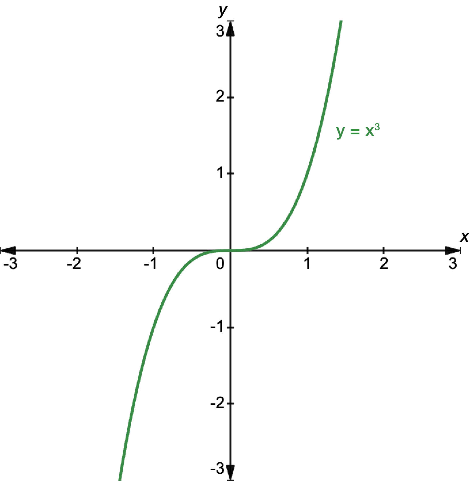
Cubic functions have the general form:
\[y=ax^{3}+bx^{2}+cx+d\]
where \(a\), \(b\), \(c\) and \(d\) are constants.
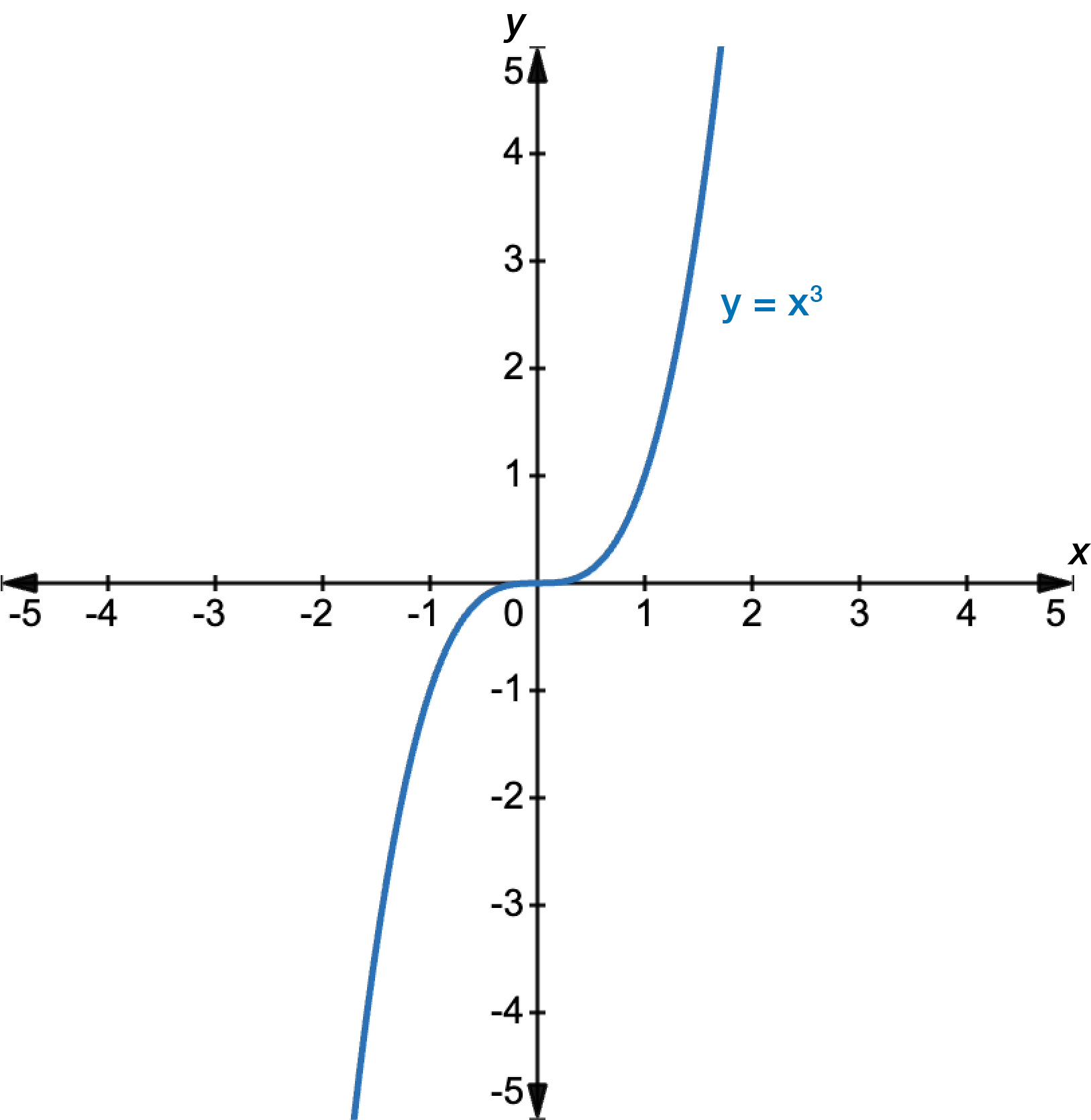
The graph for \(y=x^{3}\) goes through the origin \((0,0)\). For positive \(x\) values, the graph increases. For negative \(x\) values, the graph decreases.
Graphs of reciprocal functions
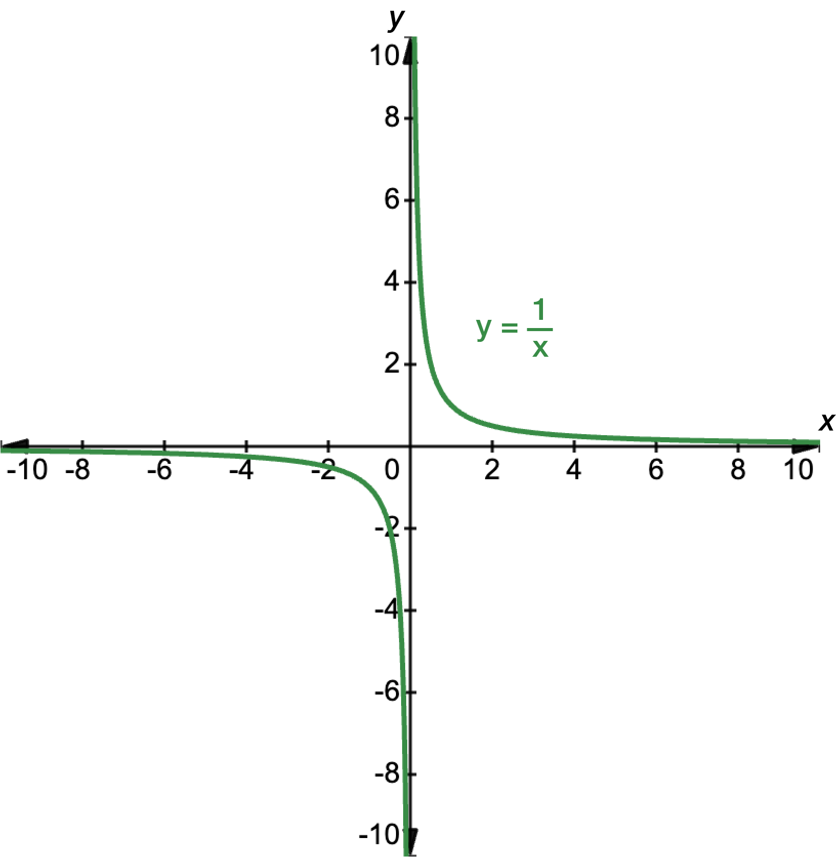
Reciprocal functions have the general form:
\[y=\dfrac{a}{x-h}+k\]
where \(a\), \(h\) and \(k\) are constants.
The graph for \(y=\dfrac{1}{y}\) has asymptotes at \(x=0\) and \(y=0\). This means that the graph approaches the \(x\)- and \(y\)-axes but never actually touches them. This goes on forever.
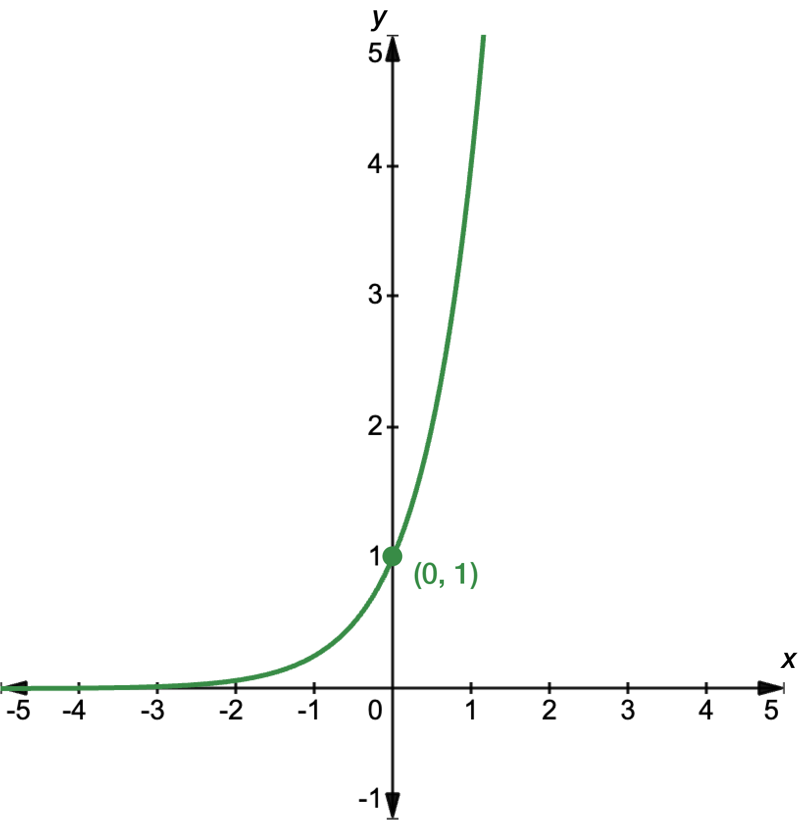
Graphs of exponential functions
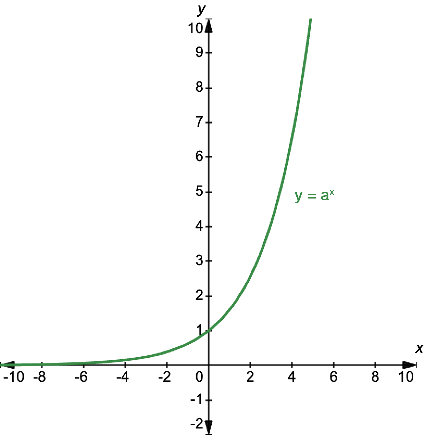
Exponential functions have the general form:
\[y=ab^{x}\]
where \(a\) is the \(y\)-intercept and \(b\) is the base that determines the rate of growth or decay. When \(b>1\), the function represents exponential growth. When \(0<b<1\), the function represents exponential decay.
The graph for \(y=1.6^{x}\) is shown. The negative \(x\)-axis is an asymptote; it approaches but never reaches \(y=0\).
Graphs of logarithmic functions
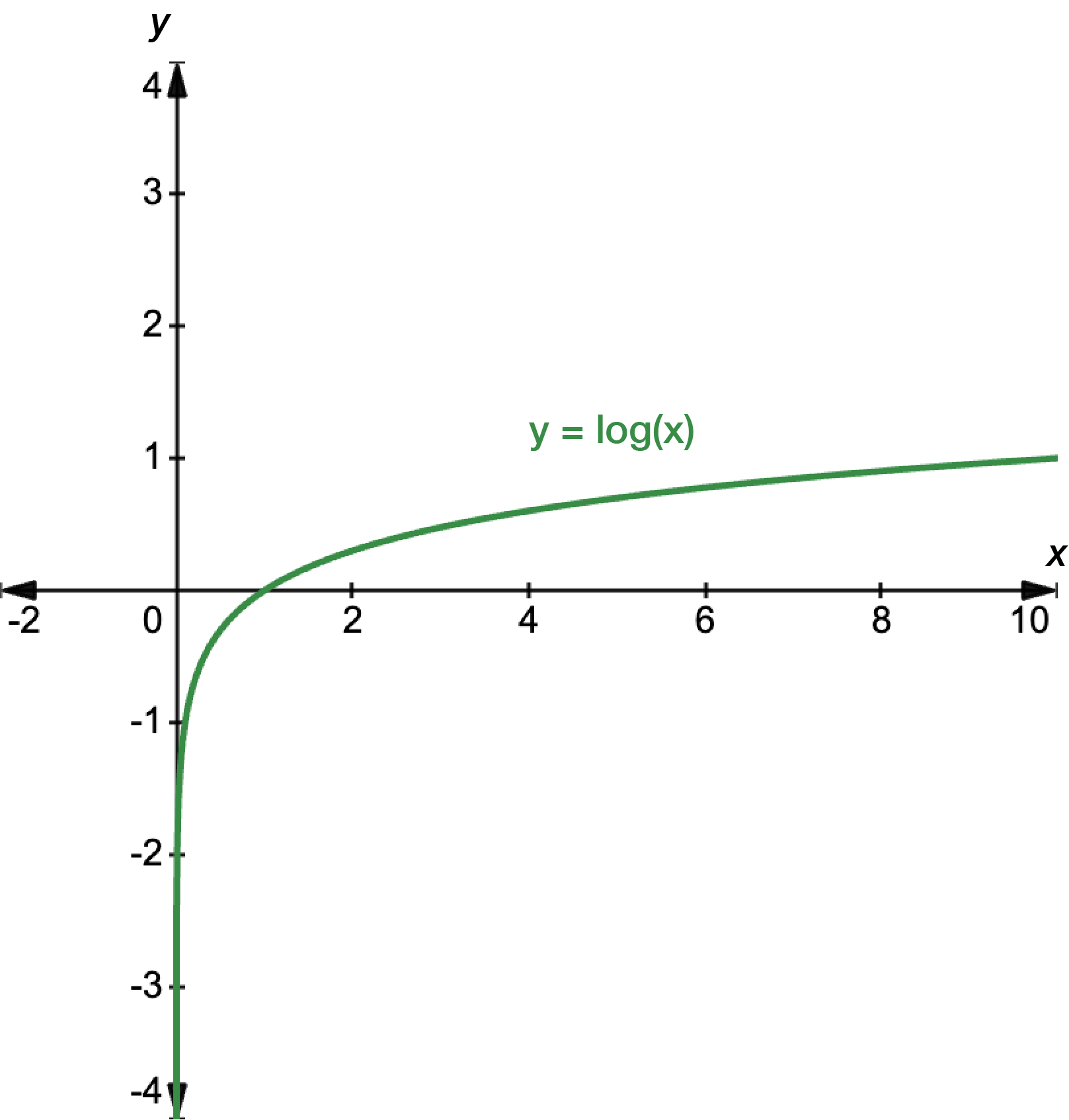
Logarithmic functions have the general form:
\[y=a\log(b(x-h))+k\]
where \(a\), \(b\), \(h\) and \(k\) are constants.
The graph of \(y=\log(x)\) has an asymptote at the \(y\)-axis; it approaches but never reaches \(x=0\). It intercepts the \(x\)-axis at \(1\) since \(\log(1)=0\).
The graphs for \(\ln(x)=\log_{e}(x)\) and any other logarithmic function look similar to this.
Transformations
Transformations of graphs involves changing the position, size, or shape of a graph by applying various modifications. These transformations can include:
reflections, where the graph is flipped over an axis
translations, where the graph is shifted up, down, left, or right
dilations, where the graph is stretched or compressed (squashed).
Graphs can also have a combination of these transformations applied.
Reflection
A reflection is a mirror image of a graph. We can reflect a graph about any line but generally, this involves the \(x\)- or \(y\)-axes.
Consider a graph given by \(y=f(x)\).
\(y=f(-x)\) reflects the graph about the \(y\)-axis.
\(y=-f(x)\) reflects the graph about the \(x\)-axis.
Example 1 – reflecting graphs
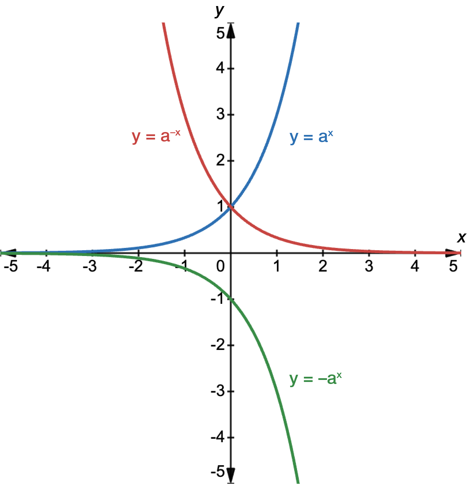
Reflect the graph of \(y=a^{x}\):
about the \(x\)-axis
about the \(y\)-axis.
The graph of \(y=a^{x}\) is shown in blue.
Reflection about the \(x\)-axis is given by \(y=a^{-x}\) in red. Reflection about the \(y\)-axis is given by \(y=-a^{x}\) in green.
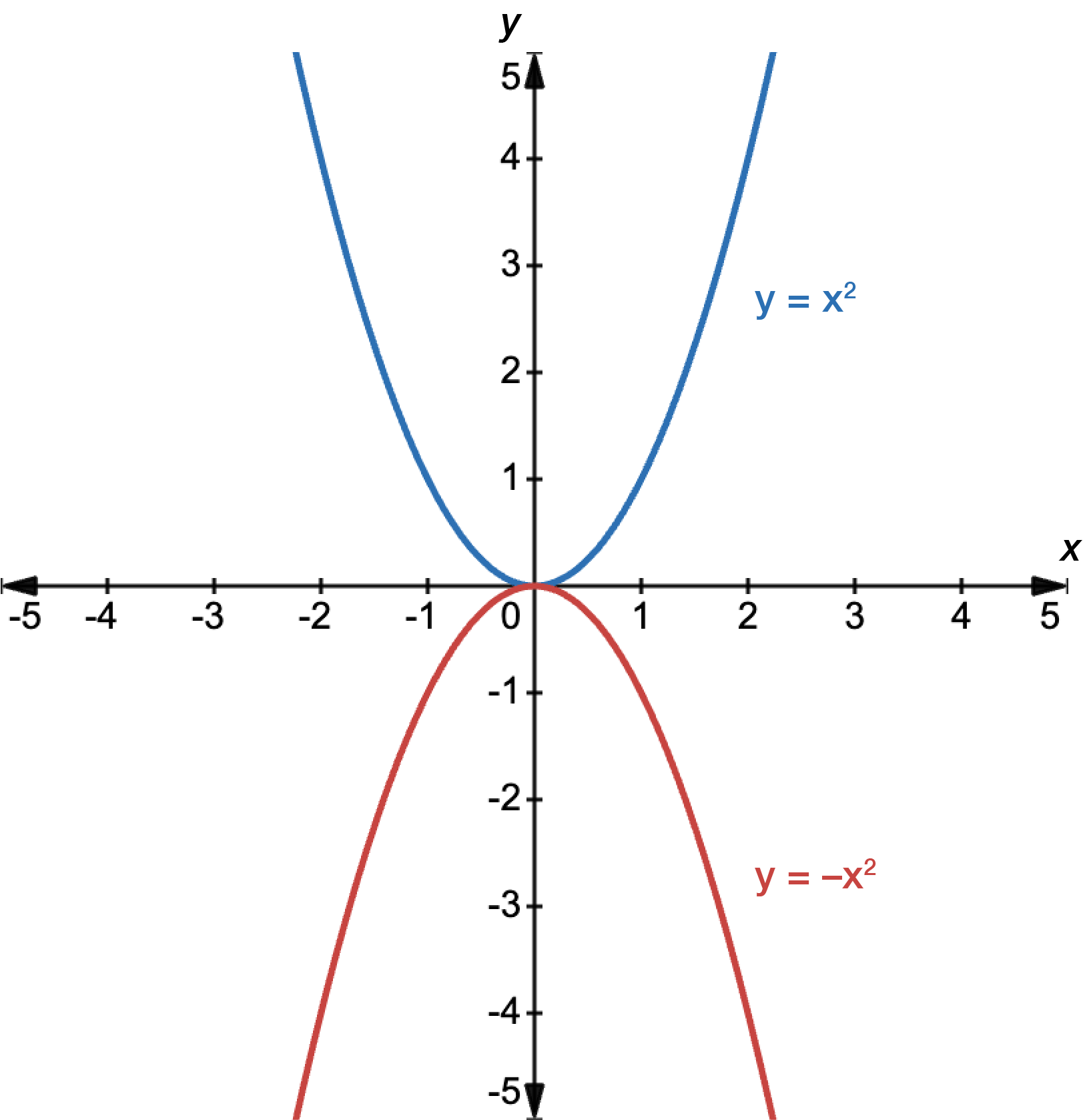
Reflect the graph of \(y=x^{2}\):
about the \(x\)-axis
about the \(y\)-axis.
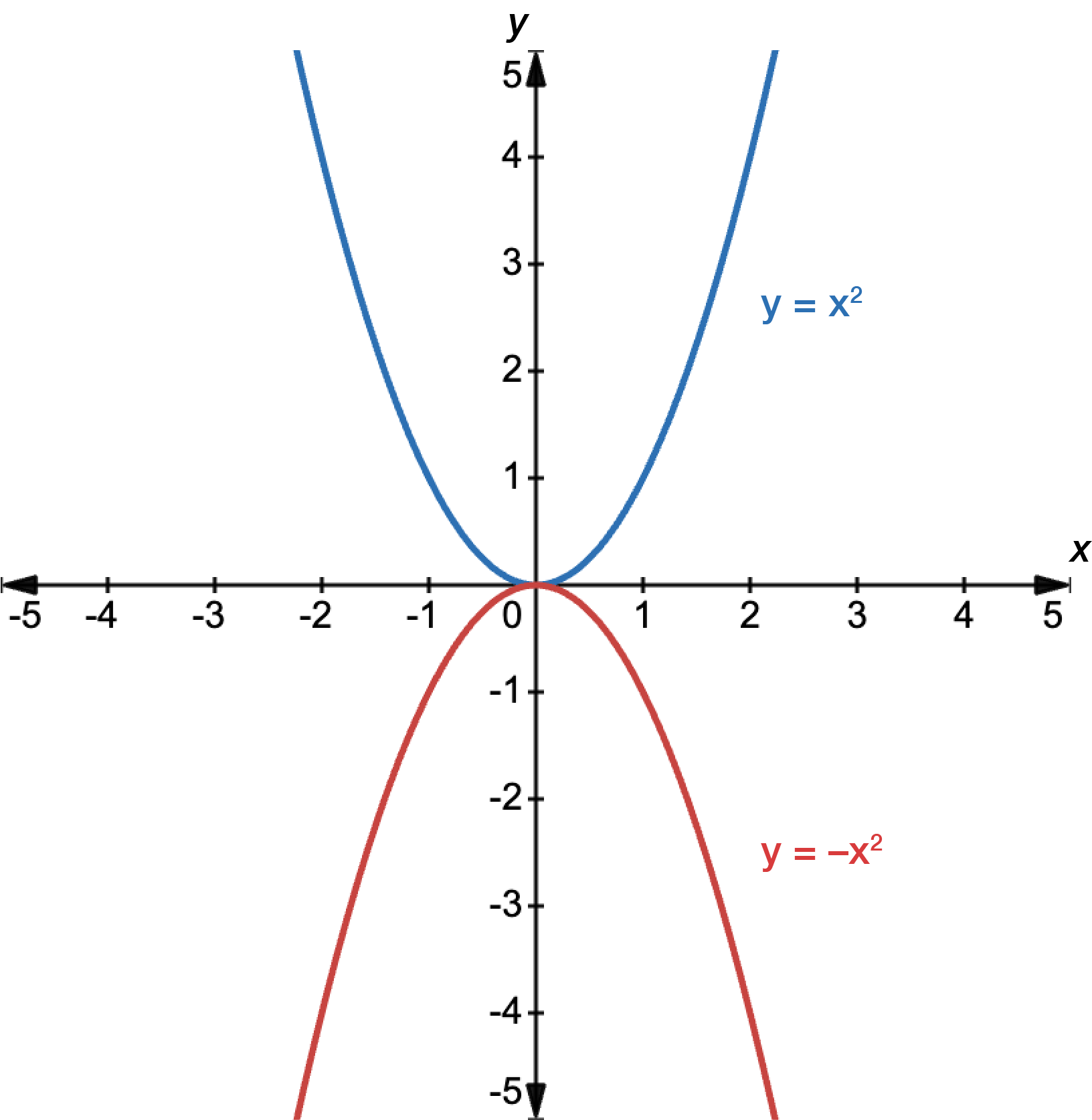
The graph of \(y=x^{2}\) is shown in blue.
Reflection about the \(x\)-axis is given by \(y=-x^{2}\) in red. Reflection about the \(y\)-axis is given by \(y=(-x)^{2}=x^{2}\), which does not change the original graph.
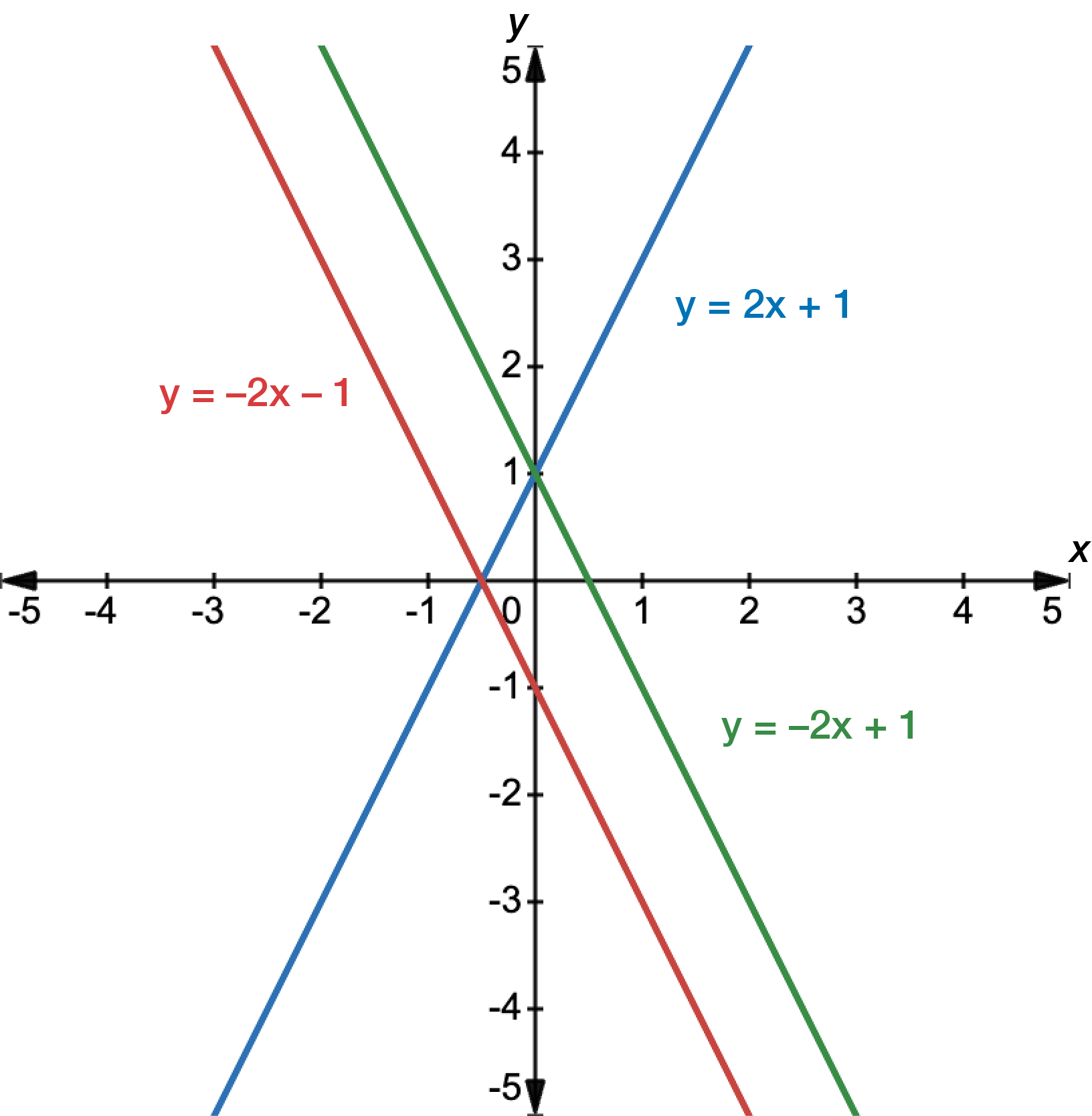
Reflect the graph of \(y=2x+1\):
about the \(x\)-axis
about the \(y\)-axis.
The graph of \(y=2x+1\) is shown in blue.
Reflection about the \(x\)-axis is given by \(y=-(2x+1)=-2x-1\) in red. Reflection about the \(y\)-axis is given by \(y=2(-x)+1=-2x+1\) in green.
Translation
Translation involves shifting a graph horizontally or vertically along the \(x-y\) plane.
For horizontal translation:
the graph of \(y=f(x-a)\) is a shift of \(y=f(x)\) \(a\) units to the right
the graph of \(y=f(x+a)\) is a shift of \(y=f(x)\) \(a\) units to the left.
For vertical translation:
the graph of \(y=f(x)+b\) is a shift of \(y=f(x)\) \(b\) units up
the graph of \(y=f(x)-b\) is a shift of \(y=f(x)\) \(b\) units down.
Example 1 – translating graphs
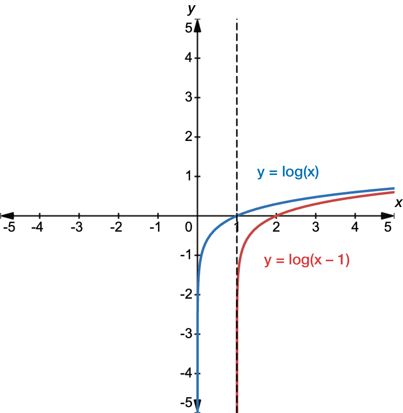
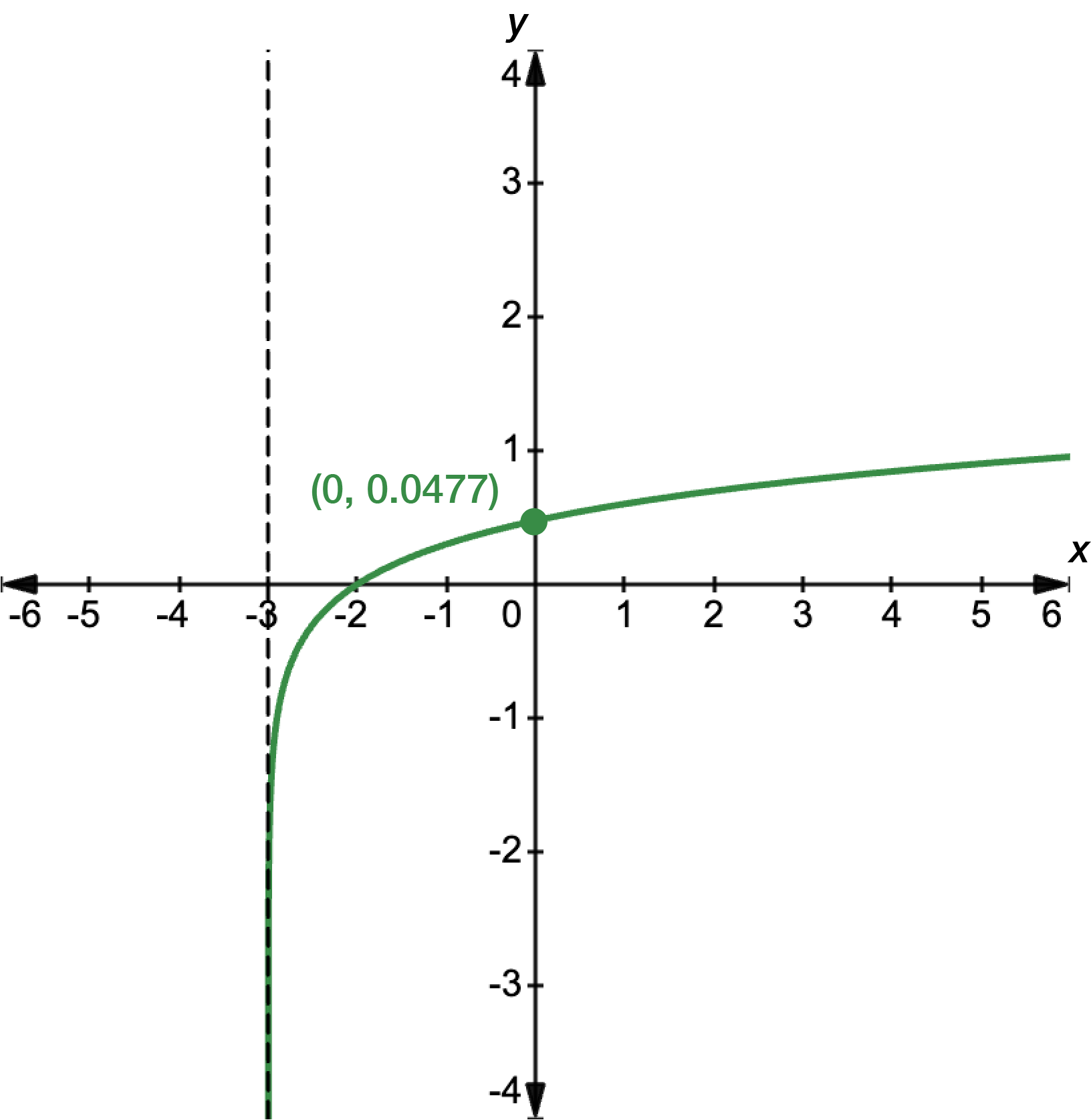
Translate \(y=\log(x)\), \(1\) unit to the right.
The graph of \(y=\log(x)\) is shown in blue. It has an asymptote at the \(y\)-axis and an \(x\)-intercept at \(x=1\).
Translation \(1\) unit to the right gives \(y=\log(x-1)\) in red. This shifts the asymptote to \(x=1\) and the \(x\)-intercept to \(x=2\). When the asymptote is not at an axis, we show it using a dashed line.
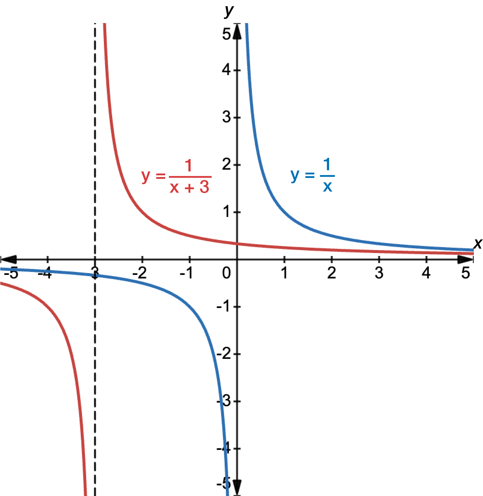
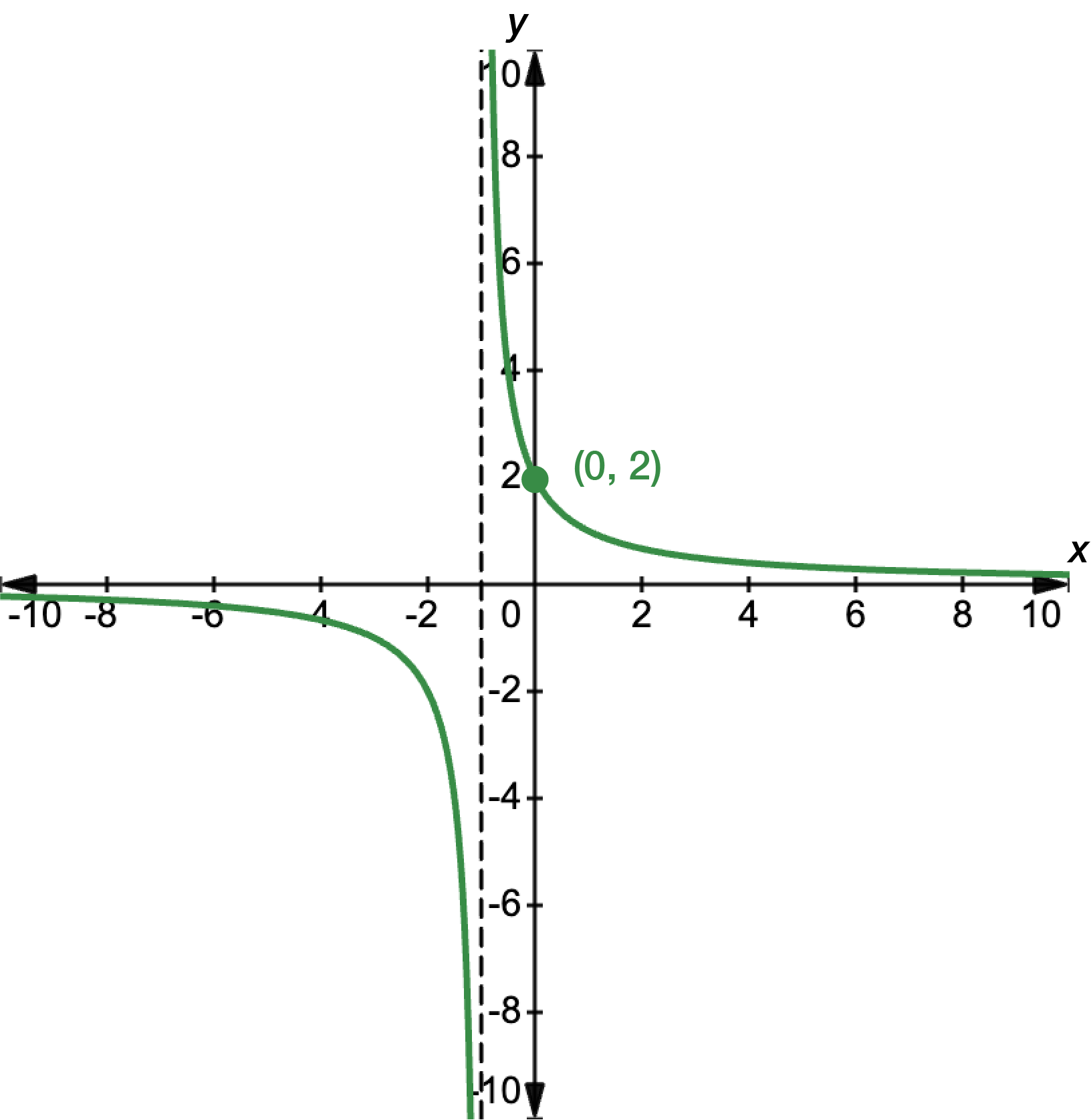
Translate \(y=\dfrac{1}{x}\), \(3\) units to the left.
The graph of \(y=\dfrac{1}{x}\) is shown in blue. It has asymptotes at the \(x\)- and \(y\)-axes.
Translation \(3\) units to the left gives \(y=\dfrac{1}{x+3}\) in red. This shifts the \(y\)-axis asymptote to \(x=-3\), which we need to show with a dashed line. The \(x\)-axis asymptote stays where it is.
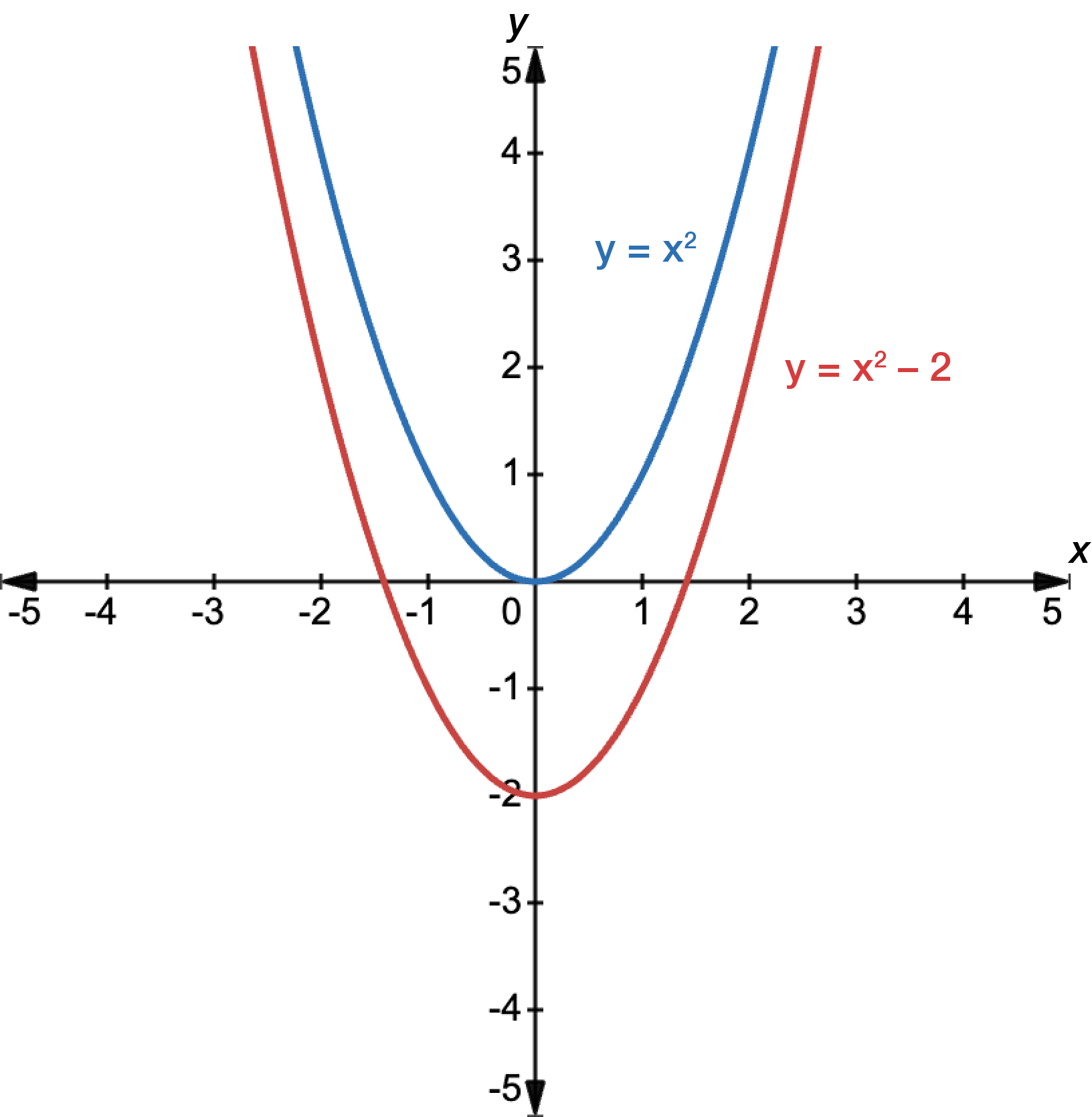
Translate \(y=x^{2}\), \(2\) units down.
The graph of \(y=x^{2}\) is shown in blue. It has a turning point at \((0,0)\).
Translation \(2\) units down gives \(y=x^{2}-2\) in red. This shifts the turning point to \((0,-2)\).
Dilation
Dilations stretch or compress a graph of a function. The stretching or compression can occur in the directions of either the \(x\)-axis, \(y\)-axis, or both.
The graph of \(y=af(x)\) is a dilation of the graph of \(y=f(x)\) by a factor of \(a\) units in the direction parallel to the \(y\)-axis. If \(a>1\), the graph is stretched. If \(a<1\), the graph is compressed or squashed.
The graph of \(y=f(bx)\) is a dilation of the graph of \(y=f(x)\) by a factor of \(\dfrac{1}{b}\) units in the direction parallel to the \(x\)-axis. If \(b>1\), the graph is compressed or squashed. If \(b<1\), the graph is stretched.
Example – dilating graphs
Dilate \(y=x^{2}\) parallel to the \(y\)-axis by a factor of:
\(4\)
\(\dfrac{1}{3}\).
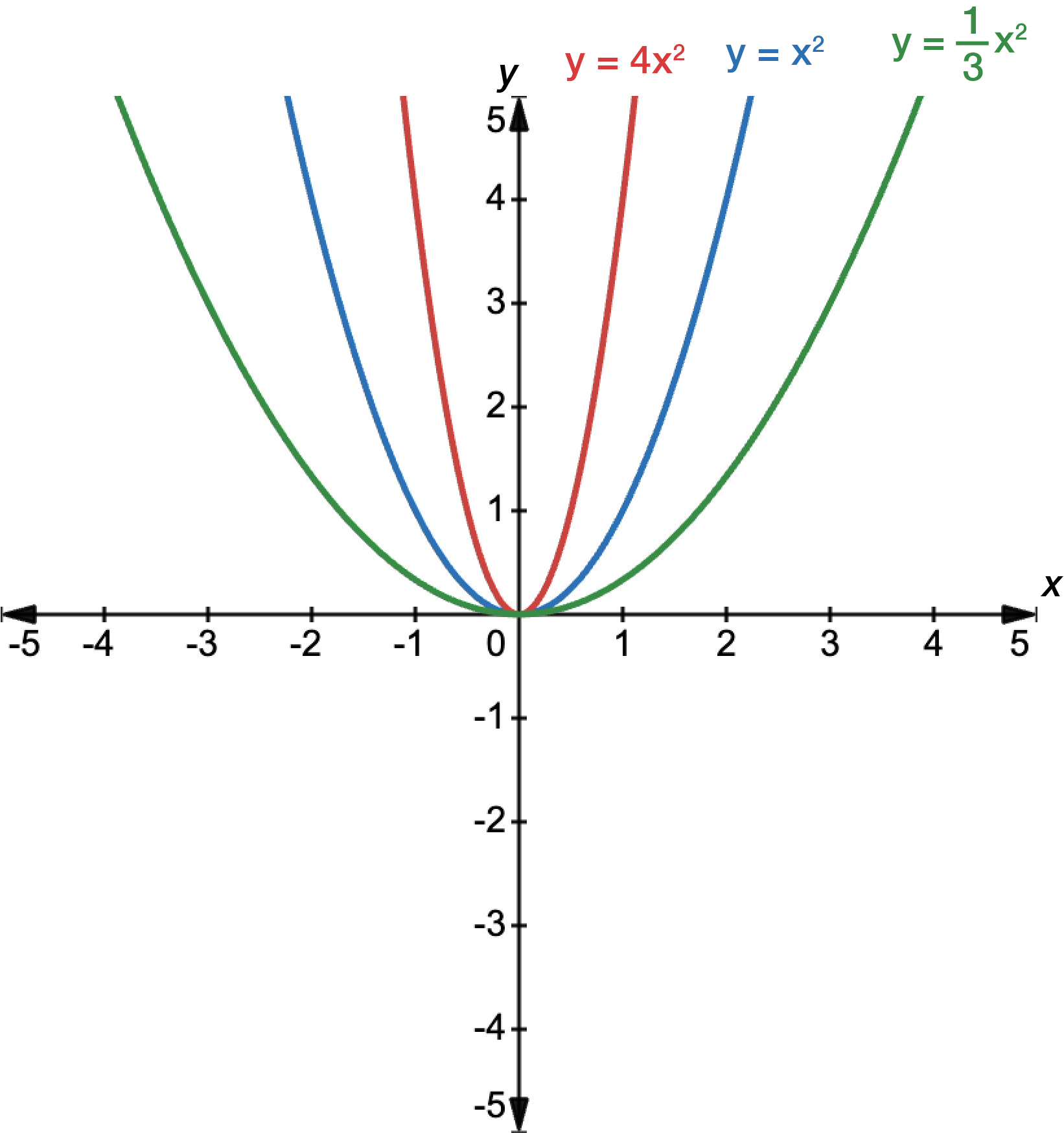
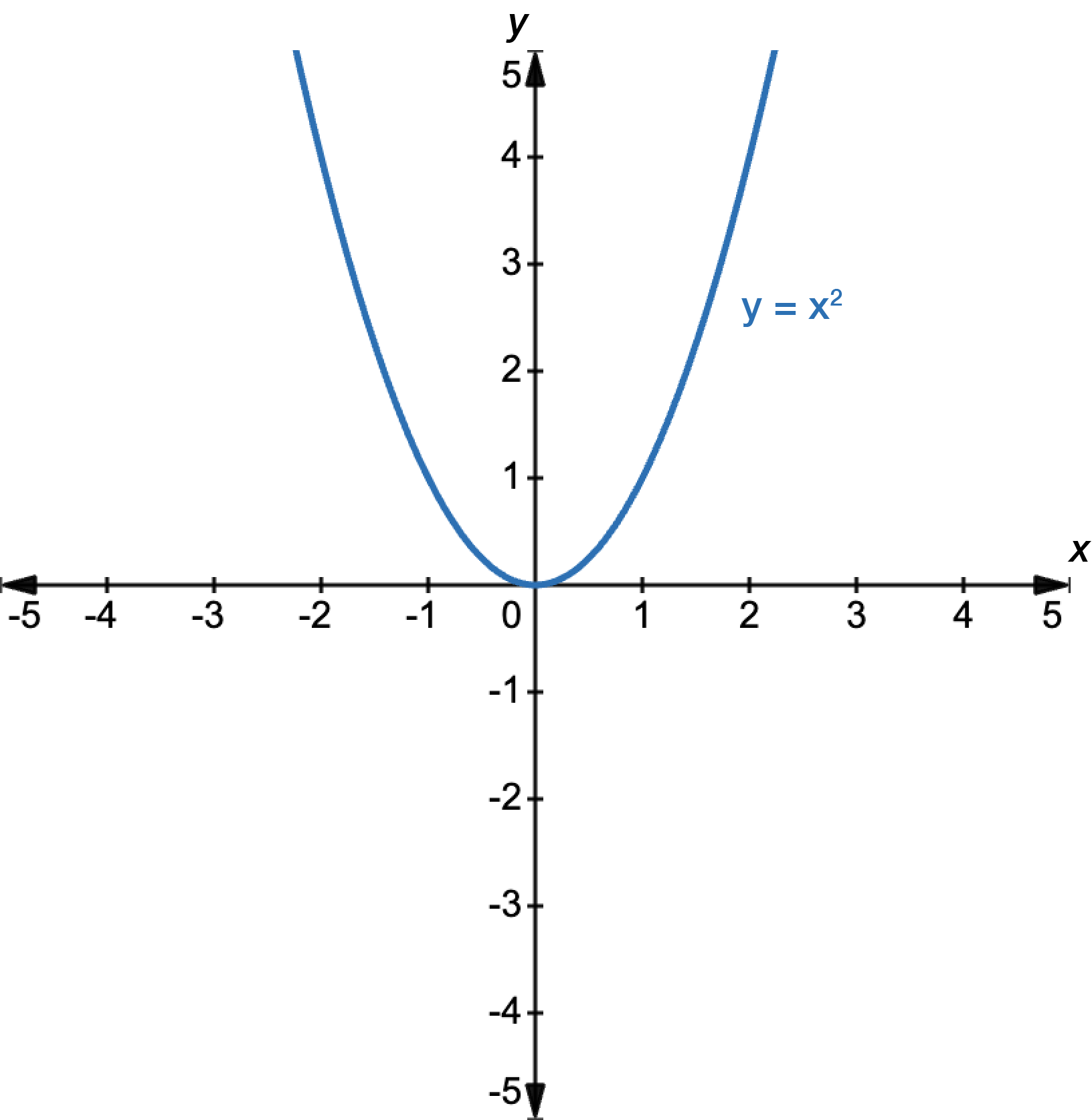
The graph of \(y=x^{2}\) is shown in blue. It has a turning point at \((0,0)\).
Dilation parallel to the \(y\)-axis by a factor of \(4\) makes the parabola appear narrower and is given by \(y=4x^{2}\) in red. Dilation parallel to the \(x\)-axis by a factor of \(\dfrac{1}{3}\) stretches the graph and is given by \(y=\dfrac{1}{3}x^{2}\) in green.
For both dilated graphs, the turning point remains unchanged at \((0,0)\), since no translation has occurred.
Combining transformations
You can get more complicated graphs by combining reflection, translation and dilation. You always start with the basic graph, then do the dilation first (if there is one), followed by translation or reflection (in any order).
Example 1 – combining transformations
Graph \(y=2x^{3}+4\).
Start by identifying the basic graph. This one is a cubic function, so the basic form is \(y=x^{3}\).
Then, we look to see what transformations have been applied.
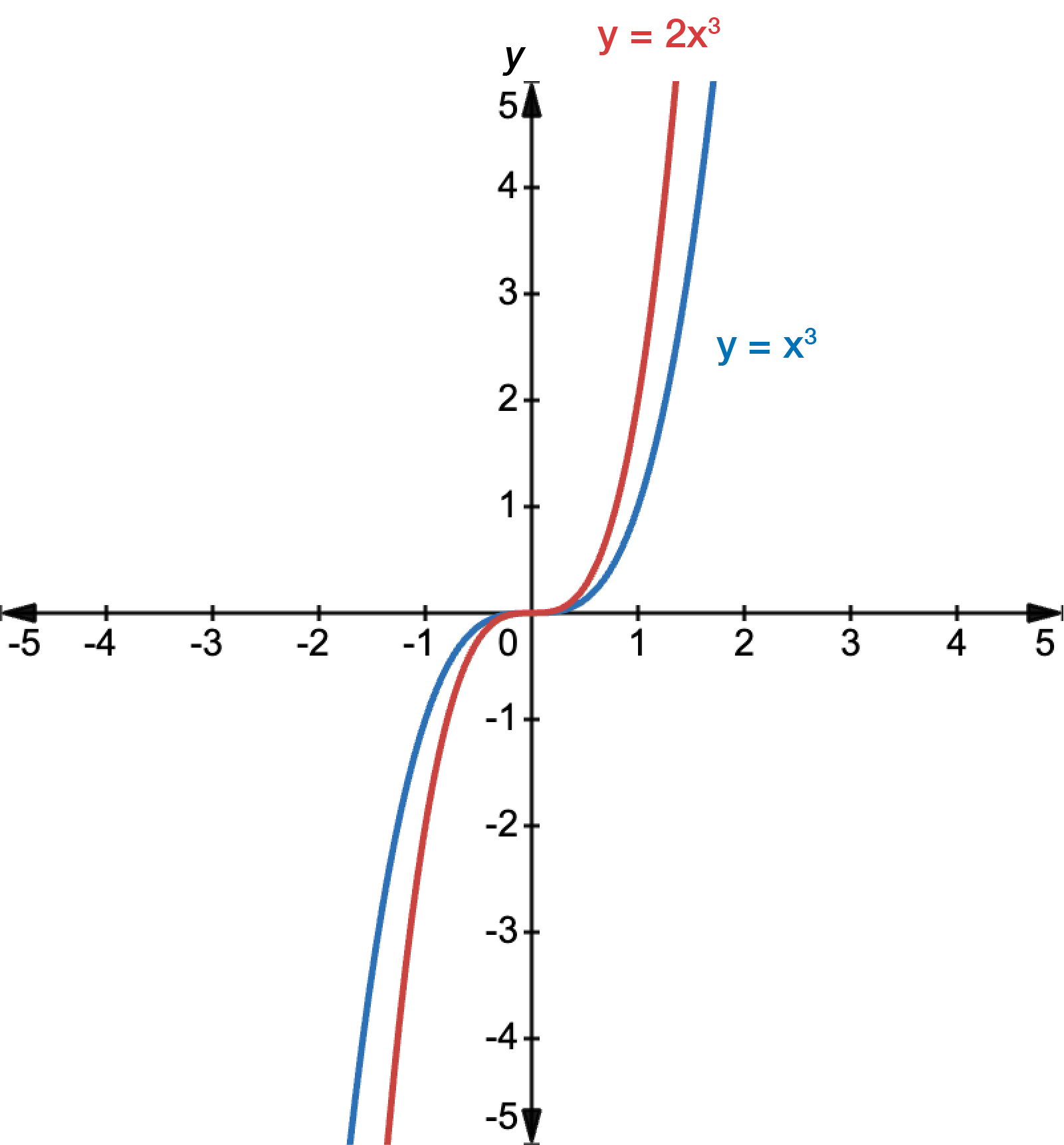
The \(2\) in front of the \(x^{3}\) is a dilation by a factor of \(2\) parallel to the \(y\)-axis. It causes the graph to compress.
The \(+4\) is a translation of \(4\) units up. It causes the graph to shift up \(4\) units.
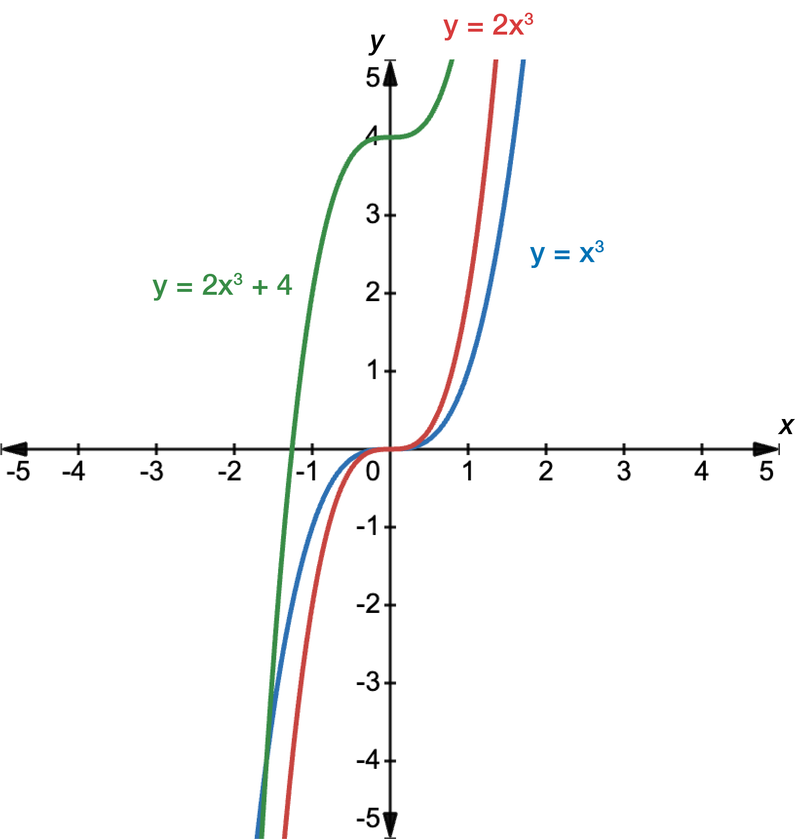
Remember that we always do the dilation first. The graph of \(y=2x^{3}\) is shown with a red line.
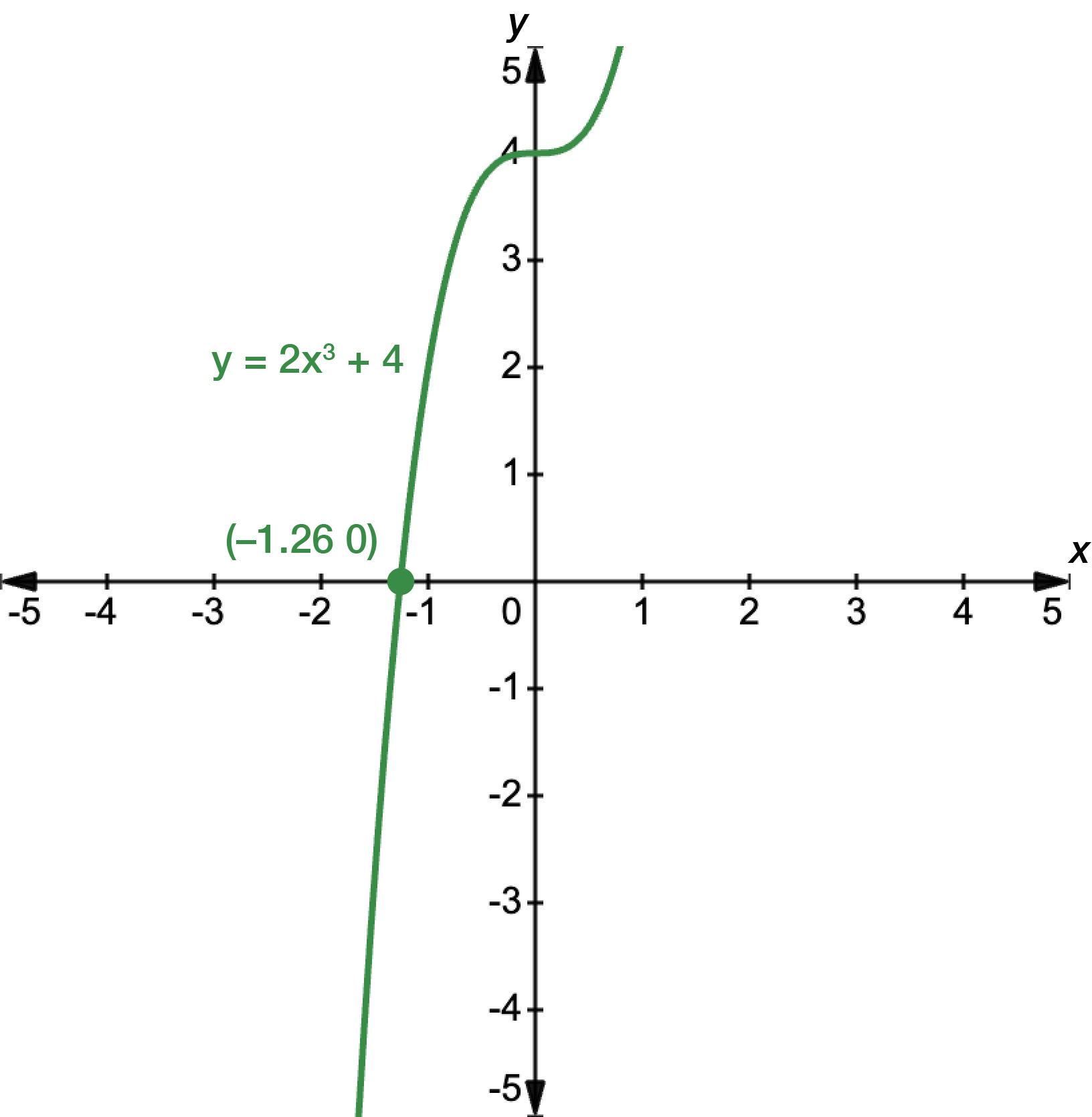
Finally, we translate the graph to get \(y=2x^{3}+4\). This is shown in green.
The only thing left to do is find the \(x\)-intercept for the new graph. Let \(y=0\).
\[\begin{align*} 2x^{3}+4 & = 0\\
2x^{3} & = -4\\
x^{3} & = -2\\
x & = -1.26
\end{align*}\]
We can add this information to the final graph.
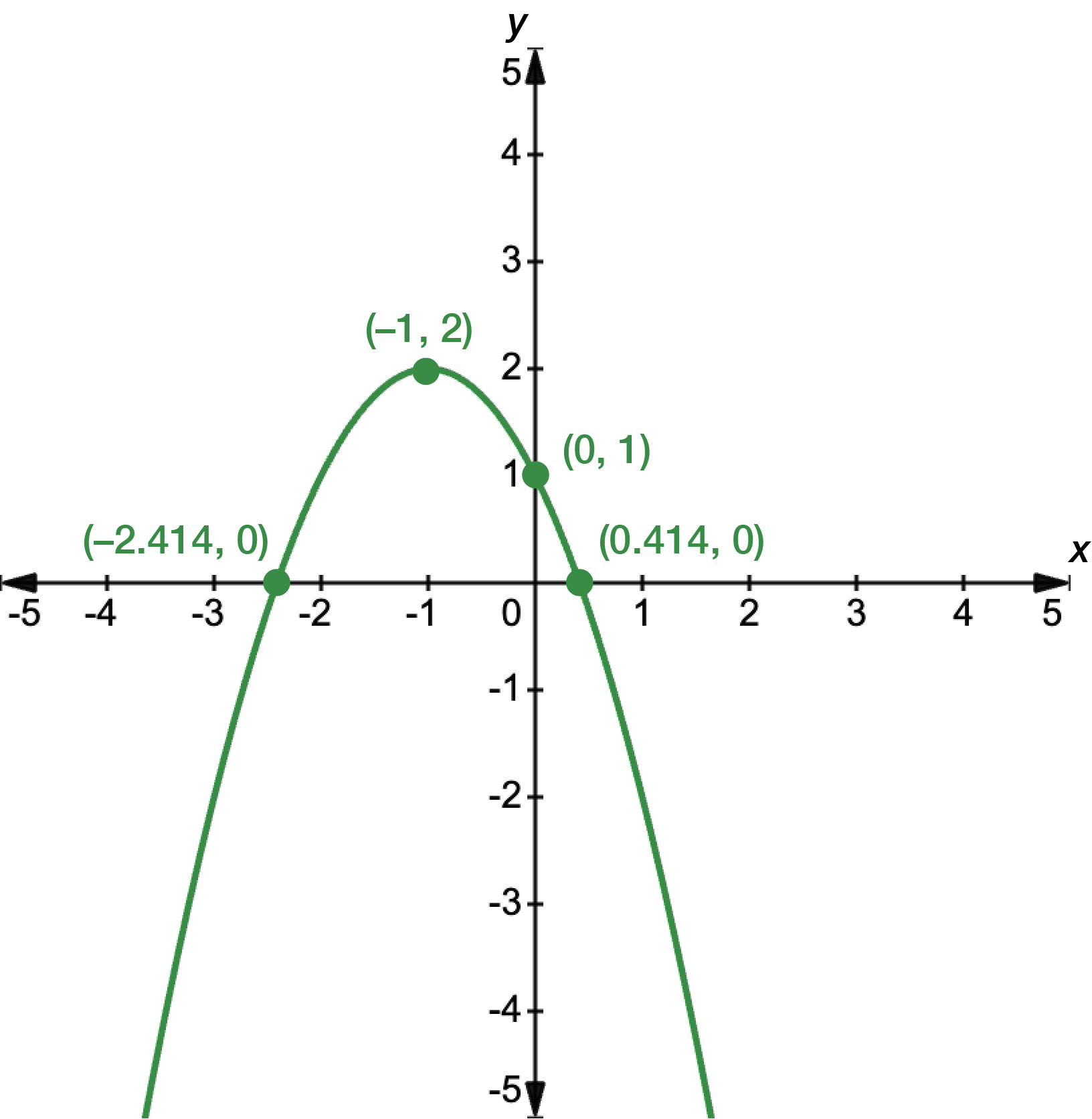
Graph \(y=-(x+2)^{2}-1\).
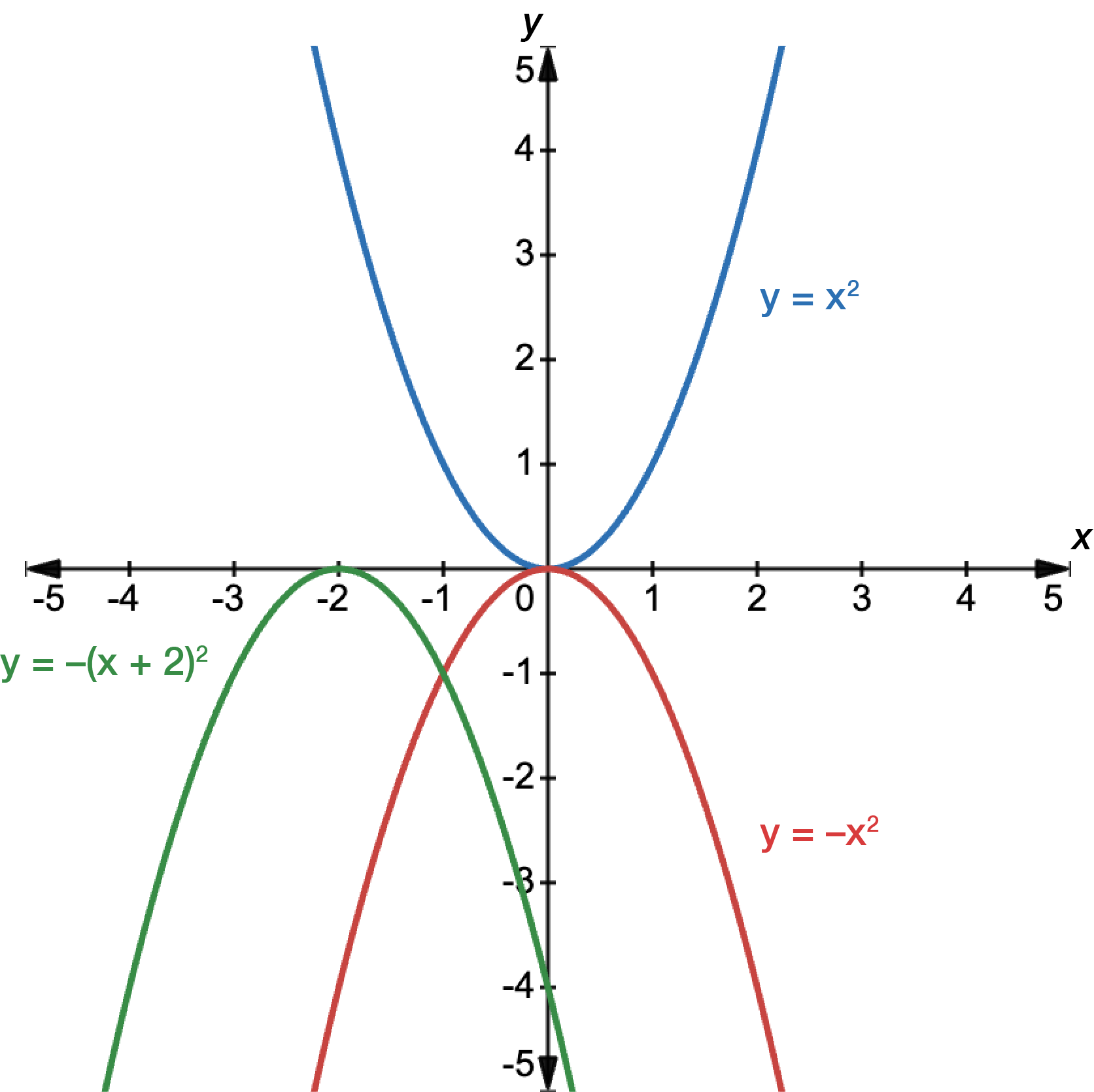
Start by identifying the basic graph. This one is a quadratic function, so the basic form is \(y=x^{2}\).
Then, we look to see what transformations have been applied.
The \(-\) in front of the \(x^{2}\) is a reflection about the \(x\)-axis.
The \(x+2\) is a translation \(2\) units to the left.
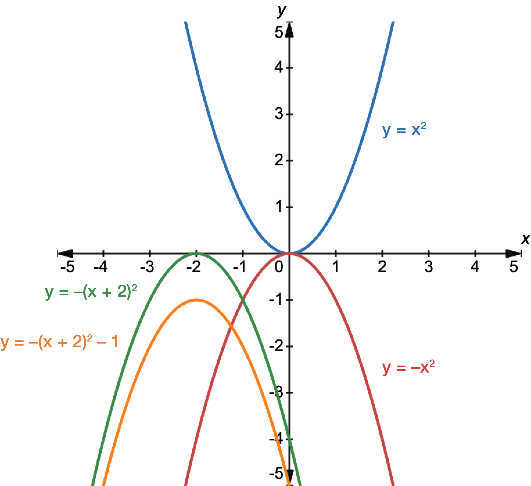
The \(-1\) is a translation of \(1\) unit down.
There is no dilation, so we can do any these transformations in any order.
Let's make our way down the list. Reflecting \(y=x^{2}\) about the \(x\)-axis gives us \(y=-x^{2}\). This is shown in a red line.
Next, we can translate the graph \(2\) units to the left. We get \(y=-(x+2)^{2}\) in green.
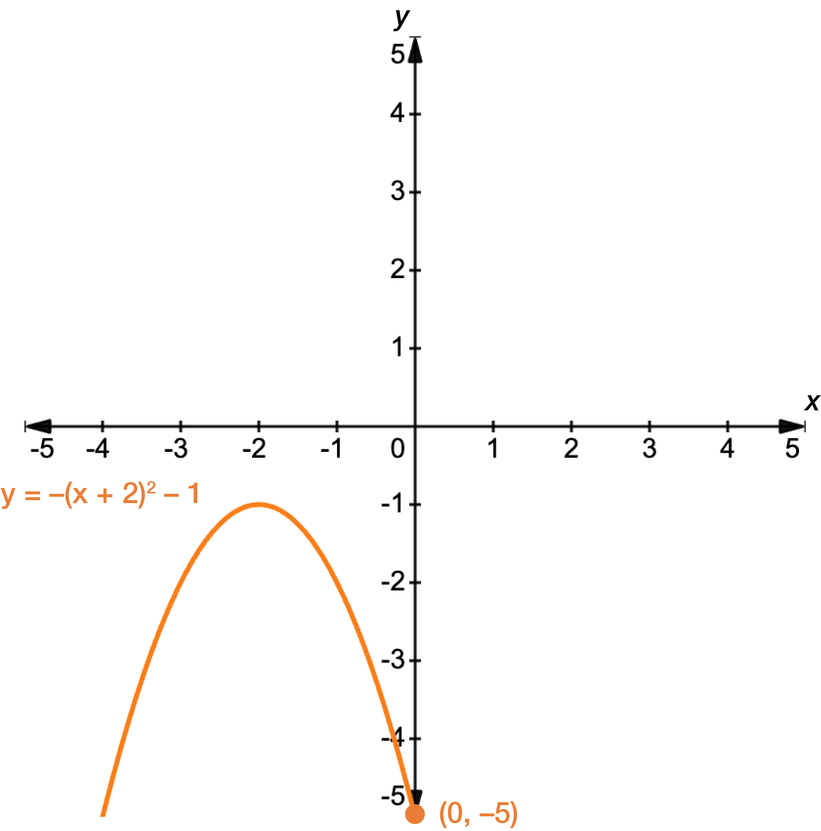
Finally, we translate the graph \(1\) unit down. This gives us \(y=-(x+2)^{2}-1\) in orange.
For quadratic functions, we should include the intercepts and turning point. The \(y\)-intercept can be found by letting \(x=0\).
\[\begin{align*} y & = -(x+2)^{2}-1\\
& = -(0+2)^{2}-1\\
& = -4-1\\
& = -5
\end{align*}\]
For the turning point, the equation is already in turning point form, so:
\[\begin{align*} y & = (x-h)^{2}+k\\
& = -(x+2)^{2}-1
\end{align*}\]
\(h=-2\) and \(k=-1\), so the turning point is at \((-2,-1)\).
We can label these points on the final graph.
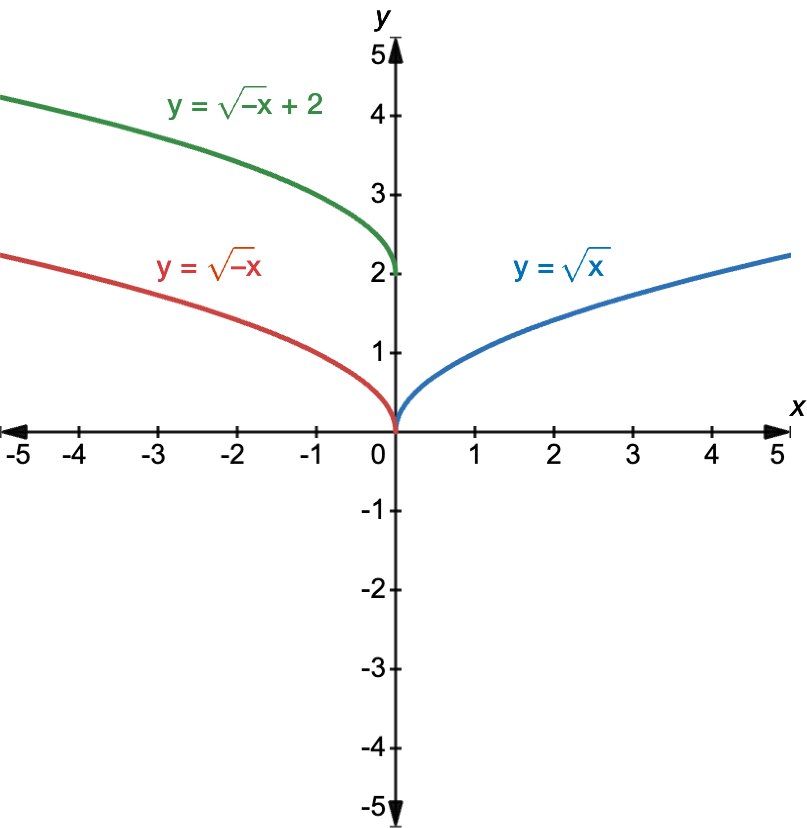
Graph \(y=\sqrt{-x}+2\).
Start by identfying the basic graph. This one is a square root, which is the same an exponential graph raised to the power of \(\dfrac{1}{2}\). The basic form is \(y=\sqrt{x}\), shown in blue.
The translations are:
\(-x\) which is a reflection of the graph about the \(y\)-axis. This gives the graph \(y=\sqrt{-x}\) shown with a red line.
\(+2\) which translates the graph \(2\) units up to give the graph \(y=\sqrt{-x}+2\). This is the final graph, shown in green.
Exercise – transforming graphs
Sketch the following graphs.
\(y=\dfrac{2}{x+1}\)
\(y=\log(x+3)\)
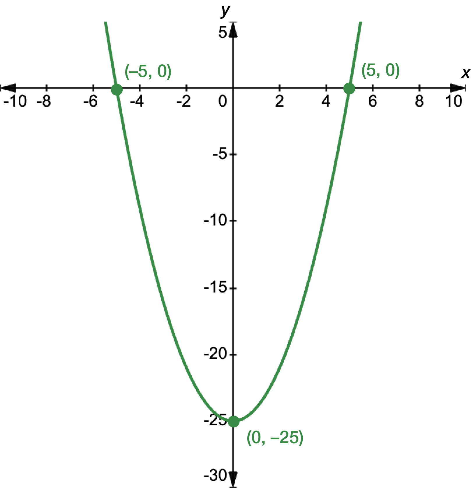
\(y=x^{2}-25\)
\(y=2-(x+1)^{2}\)
\(y=4^{x}\)
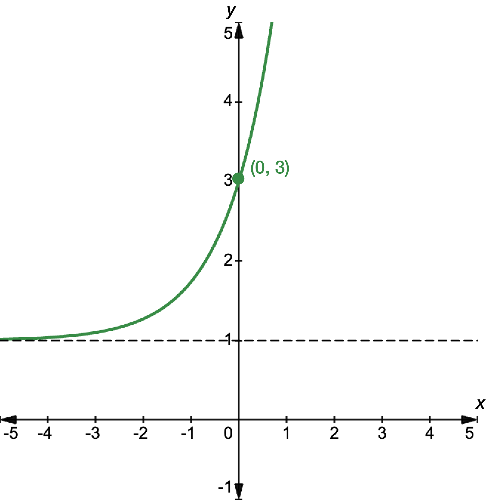
\(y=2e^{x}+1\)
\(y=\dfrac{2}{x+1}\)
\(y=\log(x+3)\)
\(y=x^{2}-25\)
\(y=2-(x+1)^{2}\)
\(y=4^{x}\)
\(y=2e^{x}+1\)
Graphs and transformations in context
In environmental science, a scientist is modelling the water level in a reservoir \(W(x)\), where \(x\) represents time in months. The base function is \(f(x)=\sin(x)\), and it needs to be transformed to reflect the real-world situation: shifted up by \(10\) units, stretched vertically by a factor of \(3\), and reflected over the \(x\)-axis. Write the transformed function.