Eigenvalues and eigenvectors

Eigenvalues and eigenvectors are important parts of an engineer’s mathematical toolbox. They give us an understanding of how buildings, structures, automobiles and materials behave in real life. But that's not all they are used for; you can see their use in many other areas of STEM, including colour theory, electric circuits, facial recognition systems, data science and quantum mechanics.

An eigenvalue is a special number, called a scalar, that is linked to a square matrix. It shows how much an eigenvector, which is a specific non-zero vector, is stretched or compressed by the matrix.

"Eigen" comes from the German word for "own", so eigenvectors and eigenvalues are vectors and values owned by the matrix.

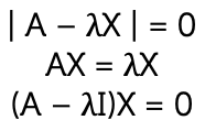
Let's consider a square, \(n\times n\) matrix called \(A\). If \(X\) is a non-zero vector of order \(n\times1\) and \(\lambda\) is a scalar, and they satisfy the equation:

\[AX = \lambda X\]

then \(\lambda\) is the eigenvalue of matrix \(A\), and \(X\) is the eigenvector.

In simpler terms, when the matrix \(A\) acts on the vector \(X\), it transforms it, and the eigenvalue \(\lambda\) tells us how much \(X\) is stretched or shrunk.

\(X\) is called a column vector (or column matrix) and is generally written as:

\[X=\left[ \begin{array}{c} x_{1}\\
x_{2}\\
\vdots\\
x_{n}
\end{array} \right] \]

This means that if \(A\) is a \(2\times2\) matrix:

\[X=\left[ \begin{array}{c} x\\
y
\end{array} \right] \]

Similarly, if \(A\) is a \(3\times3\) matrix:

\[X=\left[ \begin{array}{c} x\\
y\\
z
\end{array} \right] \]

Finding eigenvalues for \(2\times2\) matrices

To find the eigenvalue for a square matrix \(A\), we solve the characteristic equation.

\[\det \left[ A-\lambda I \right] = \left| A-\lambda I \right| = 0 \]

If \(A\) is an \(n\times n\) matrix, there will be at most \(n\) distinct eigenvalues of \(A\).

Example 1 – finding eigenvalues for \(2\times2\) matrices

Find the eigenvalues of the matrix:
\[A = \left[ \begin{array}{cc} -4 & -2\\
3 & 3
\end{array} \right] \]

We need to find the characteristic equation for matrix \(A\). It includes the \(2\times2\) identity matrix.

\[I = \left[ \begin{array}{cc} 1 & 0\\
0 & 1
\end{array} \right] \]

We can substitute this into \(A-\lambda I\).

\[\begin{align*} A-\lambda I & = \left[ \begin{array}{cc} -4 & -2\\
3 & 3
\end{array} \right]-\lambda \left[ \begin{array}{cc} 1 & 0\\
0 & 1
\end{array} \right]\\
& = \left[ \begin{array}{cc} -4 & -2\\
3 & 3
\end{array} \right]-\left[ \begin{array}{cc} \lambda & 0\\
0 & \lambda
\end{array} \right]\\
& = \left[ \begin{array}{cc} -4-\lambda & -2\\
3 & 3-\lambda
\end{array} \right]
\end{align*}\]

To find the eigenvalues, we solve \(\det[A-\lambda I]=\left|A-\lambda I\right|=0\).

\[\begin{align*} \det \left[ A-\lambda I\right] & = 0\\ \det \left[ \begin{array}{cc} -4-\lambda & -2\\
3 & 3-\lambda \end{array} \right] & = 0\\
\left( -4-\lambda \right)\left( 3-\lambda \right) -3 \left( -2 \right) & = 0\\
-12+4\lambda-3\lambda+\lambda^{2}+6 & = 0\\
\lambda^{2}+\lambda-6 & = 0
\end{align*}\]

The characteristic equation that forms is a quadratic equation, which we can factorise and use the null factor law or quadratic formula to solve.

\[\begin{align*} 0 & = \lambda^{2}-\lambda-6\\
& = \left( \lambda+3\right) \left( \lambda-2\right)
\end{align*}\] \[\begin{align*} \lambda+3 & = 0\\
\lambda & = -3
\end{align*}\] \[\begin{align*} \lambda-2 & = 0\\
\lambda & = 2
\end{align*}\]

The \(2\times2\) matrix \(A\) has two eigenvalues: \(\lambda_{1}=-3\) and \(\lambda_{2}=2\).

Finding eigenvectors for \(2\times2\) matrices

Each eigenvalue of a matrix has a corresponding eigenvector. To find the eigenvectors, we solve the following equation for each eigenvalue:

\[\begin{align*} AX & =\lambda X\\
AX-\lambda X & = 0\\
(A-\lambda I)X & = 0
\end{align*} \]

In the very last line, you might notice that we have not written \((A-\lambda)X=0\). This wouldn't make sense, because \(A\) is an \(n\times n\) matrix and \(\lambda\) is a scalar (number). We cannot subtract a number from a matrix, so we need to complete a transformation in which we multiply by the identity matrix.

For each eigenvalue, \(\lambda\), solve the following to obtain the eigenvector, \(X\):
\[(A-\lambda I)X=0\]

A multiple of any eigenvector is an eigenvector. We do not consider \(\vec{X}=\vec{0}\) to be an eigenvector.

Example 1 – finding eigenvectors for \(2\times2\) matrices

Find the eigenvectors of the matrix:
\[A = \left[ \begin{array}{cc} -4 & -2\\
3 & 3
\end{array} \right]\]

This is the same matrix as Example 1 – finding eigenvectors for \(2\times2\) matrices, so we already know that the eigenvalues are \(\lambda_{1}=-3\) and \(\lambda_{2}=2\).

To find the corresponding eigenvectors, we solve \((A-\lambda I)X=0\) for \(X\). We can write \(X\) in the form \(\left[ \begin{array}{c} x\\ y \end{array} \right]\) and substitute all of these into the equation.

\[ \left[ \begin{array}{cc} -4-\lambda & -2\\
3 & 3-\lambda
\end{array} \right]
\left[ \begin{array}{c} x\\
y
\end{array} \right] = 0 \]

For \(\lambda_{1}=-3\):

\[\begin{align*} \left[ \begin{array}{cc} -4-(-3) & -2\\
3 & 3-(-3)
\end{array} \right]
\left[ \begin{array}{c} x\\
y
\end{array} \right] & = 0\\
\left[ \begin{array}{cc} -1 & -2\\
3 & 6
\end{array} \right]
\left[ \begin{array}{c} x\\
y
\end{array} \right] & = 0
\end{align*}\]

This gives two linear equations:

\[\begin{align*} -x-2y & = 0\\
3x+6y & = 0
\end{align*}\]

These cannot be solved to give a unique solution, as one is a multiple of the other. This means there are an infinite number of solutions.

Remember that when you encounter this case, you have to let one variable be free. We can let \(y=t\) where \(t\in\mathbb{R}\). This gives us \(x=-2t\) and \(y=t\), which we can substitute into the general eigenvector form:

\[\begin{align*} \left[ \begin{array}{c} x\\
y
\end{array} \right] & = \left[ \begin{array}{c} -2t\\
t
\end{array} \right]\\
& = t \left[ \begin{array}{c} -2\\
1
\end{array} \right]
\end{align*}\]

As \(t\) can be any number, there are an infinite number of eigenvectors. However, the convention is that we recognise any eigenvector multiplied by a scalar is still an eigenvector and we state the eigenvector in the lowest possible terms. So, the eigenvector that corresponds to \(\lambda_{1}=-3\) is:

\[\begin{align*} X_{1} & = \left[ \begin{array}{c} -2\\
1
\end{array} \right]
\end{align*}\]

For \(\lambda_{2}=2\):

\[\begin{align*} \left[ \begin{array}{cc} -4-2 & -2\\
3 & 3-2
\end{array} \right] \left[ \begin{array}{c} x\\
y \end{array} \right] & = 0\\
\left[ \begin{array}{cc} -6 & -2\\
3 & 1
\end{array} \right] \left[ \begin{array}{c} x\\
y
\end{array} \right] & = 0\end{align*}\]

This gives two linear equations:

\[\begin{align*} -6x-2y & = 0\\
3x+y & = 0
\end{align*}\]

Again, we see that the one equation is a multiple of the other. Let's let \(x=t\), which gives us \(y=-3t\) where \(t\in\mathbb{R}\). We can substitute \(x\) and \(y\) into the eigenvector :

\[\begin{align*} \left[ \begin{array}{c} x\\
y \end{array} \right] & = \left[ \begin{array}{c} t\\
-3t
\end{array}\right]\\
& = t\left[\begin{array}{c} 1\\
-3 \end{array} \right]
\end{align*}\]

In lowest terms, the eigenvalue corresponding to \(\lambda_{2}=2\) is:

\[X_{2} = \left[ \begin{array}{c} 1\\
-3
\end{array} \right] \]

Your turn – finding eigenvalues and eigenvectors for \(2\times2\) matrices

1. Find the eigenvalues and eigenvectors for the following matrices.
1. \(\left[ \begin{array}{cc} 2 & 1\\
   1 & 2
   \end{array} \right] \)
2. \(\left[ \begin{array}{cc} 4 & -1\\
   1 & 2
   \end{array} \right] \)
3. \(\left[ \begin{array}{cc} -1 & -3\\
   1 & 3
   \end{array} \right] \)

Eigenvalues and eigenvectors for \(3\times3\) matrices

Regardless of the size of the matrix, the method for finding eigenvalues and eigenvectors is the same.

The working out is quite long for these types of questions, but as long as you work through them carefully and follow the correct method, you will reach the correct answer.

Example 1 – finding eigenvalues and eigenvectors for \(3\times3\) matrices

Find the eigenvalues and eigenvectors of the matrix:
\[B = \left[ \begin{array}{ccc} 1 & 1 & -2\\
-1 & 0 & 1\\
-2 & 1 & 1
\end{array} \right]\]

We can find the eigenvalues by solving \(\det\left[B-\lambda I\right]\).

This is the characteristic equation. It is a cubic polynomial. The degree of the polynomial is generally the same as \(n\) for a \(n\times n\) matrix.

We factorise the characteristic equation to solve it.

\[\begin{align*} -\lambda^{3} + 2\lambda^{2} + 3\lambda & = 0\\
-\lambda(\lambda^{2}-2\lambda-3) & = 0\\
-\lambda(\lambda-3)(\lambda+1) & = 0
\end{align*}\]

Hence, the eigenvalues of \(B\) are \(\lambda_{1}=0\), \(\lambda_{2}=3\) and \(\lambda_{3}=-1\).

To find the eigenvectors for each eigenvalue, we solve \((A-\lambda I)X=0\). In this case, since the order of the matrix is \(3\times3\), \(X = \left[ \begin{array}{c} x\\ y\\ z \end{array} \right]\). Here, we haven't showed all of the steps.

For \(\lambda_{1}=0\):

\[\begin{align*} \left(B-\lambda I\right)X & = 0\\ \left[ \begin{array}{ccc} 1-0 & 1 & -2\\
-1 & 0-0 & 1\\
-2 & 1 & 1-0
\end{array} \right]
\left[ \begin{array}{c} x\\
y\\
z
\end{array} \right] & = 0\\
\left[ \begin{array}{ccc} 1 & 1 & -2\\
-1 & 0 & 1\\
-2 & 1 & 1
\end{array} \right]
\left[ \begin{array}{c} x\\
y\\
z
\end{array} \right] & = 0\\
x+y-2z & = 0\\
-x+z & = 0\\
-2x+y+z & = 0
\end{align*}\]

From the second equation, we get \(z=x\).

We can substitute this into the first equation:

\[\begin{align*} x+y-2z & = 0\\
x+y-2(x) & = 0\\
y-x & = 0\\
y & = x
\end{align*}\]

Since \(x=y=z\), we can let them \(=t\), where \(t\in\mathbb{R}\). The eigenvector is therefore:

\[\begin{align*} X & = \left[ \begin{array}{c} t\\
t\\
t
\end{array} \right]\\
& = t \left[ \begin{array}{c} 1\\
1\\
1
\end{array} \right]
\end{align*} \]

In its lowest form, \(X_{1} = \left[ \begin{array}{c} 1\\ 1\\ 1 \end{array} \right] \).

For \(\lambda_{2}=3\):

\[\begin{align*} \left(B-\lambda I\right)X & = 0\\
\left[ \begin{array}{ccc} 1-3 & 1 & -2\\
-1 & 0-3 & 1\\
-2 & 1 & 1-3
\end{array} \right]
\left[ \begin{array}{c} x\\
y\\
z
\end{array} \right] & = 0\\
\left[ \begin{array}{ccc} -2 & 1 & -2\\
-1 & -3 & 1\\
-2 & 1 & -2
\end{array} \right]
\left[ \begin{array}{c} x\\
y\\
z
\end{array}\right] & = 0\\
-2x+y-2z & = 0\\
-x-3y+z & = 0 \\
-2x+y-2z & = 0
\end{align*}\]

The first and third equations are identical, so we can pick just the first and second to solve. We can let \(z=t\), where \(t\in\mathbb{R}\).

\[\begin{align*} -2x+y & = 2t\\
-x-3y & = -t
\end{align*}\]

We can multiply the second equation by \(2\) and subtract from the first equation to get:

\[\begin{align*} -2x+y - 2(-x-3y) & = 2t-(2\times(-t))\\
-2x+y+2x+6y & = 2t+2t\\
7y & = 4t\\
y & = \frac{4}{7}t
\end{align*}\]

We can then multiply the first equation by \(3\) and add it to the second equation to get:

\[\begin{align*} 3(-2x+y) + (-x-3y) & = 3(2t) + (-t)\\
-6x+3y-x-3y & = 6t-t\\
-7x & = 5t\\
x & = -\frac{5}{7}t
\end{align*}\]

Thus, \(y=\dfrac{4}{7}t\) and \(x=-\dfrac{5}{7}t\).

Hence, the eigenvector has the form:

\[\begin{align*} X & = \left[ \begin{array}{c} -\frac{5}{7}t\\
\frac{4}{7}t\\
-\frac{5}{7}t
\end{array} \right] \\
& = t\left[ \begin{array}{c} -\frac{5}{7}\\
\frac{4}{7}\\
1
\end{array}\right]
\end{align*}\]

To get the lowest form, we can make \(t=7\) to get rid of the fraction. Hence, \(X_{2} = \left[ \begin{array}{c} -5\\ 4\\ 7 \end{array} \right]\) or \(\left[ \begin{array}{c} 5\\ -4\\ -7 \end{array} \right]\).

For \(\lambda_{3}=-1\):

\[\begin{align*} \left(B-\lambda I\right)X & = 0\\
\left[ \begin{array}{ccc} 1-(-1) & 1 & -2\\
-1 & 0-(-1) & 1\\
-2 & 1 & 1-(-1)
\end{array} \right]
\left[
\begin{array}{c} x\\
y\\
z
\end{array} \right] & = 0\\
\left[ \begin{array}{ccc} 2 & 1 & -2\\
-1 & 1 & 1\\
-2 & 1 & 2
\end{array} \right]
\left[ \begin{array}{c} x\\
y\\
z
\end{array}\right] & = 0\\
2x+y-2z & = 0\\
-x+y+z & = 0\\
-2x+y+2z & = 0
\end{align*}\]

We can add the first equation to the third equation to get:

\[\begin{align*} 2x+y-2z + (-2x+y+2z) & = 0+0\\
2x+y-2z-2x+y+2z & = 0\\
2y & = 0\\
y & = 0
\end{align*}\]

We can substitute \(y=0\) into the second equation:

\[\begin{align*} -x+y+z & = 0\\
-x+0+z & = 0\\
x & = z
\end{align*}\]

We can then let \(z=t\), where \(t\in\mathbb{R}\), so that the eigenvector has the form:

\[\begin{align*} X & = \left[ \begin{array}{c} t\\
0\\
t
\end{array} \right]\\
& = t \left[ \begin{array}{c} 1\\
0\\
1
\end{array} \right]
\end{align*}\]

This gives us the lowest form, \(X_{3} = \left[ \begin{array}{c} 1\\ 0\\ 1 \end{array} \right] \).

In summary, the eigenvalues of matrix \(B\) are \(\lambda_{1}=0\), \(\lambda_{2}=3\) and \(\lambda_{3}=-1\). The corresponding eigenvectors are \(X_{1}=\left[ \begin{array}{c} 1\\ 1\\ 1 \end{array} \right]\), \(X_{2}=\left[ \begin{array}{c} 5\\ -4\\ -7 \end{array} \right]\) and \(X_{3}=\left[ \begin{array}{c} 1\\ 0\\ 1 \end{array} \right]\).

Your turn – finding eigenvalues and eigenvectors for \(3\times3\) matrices

1. Determine which of the following are eigenvectors of the matrix \(A = \left[ \begin{array}{ccc} 2 & 0 & -1\\
   0 & 1 & 0\\
   4 & 0 & 2
   \end{array} \right]\)
1. \(\left[ \begin{array}{c} 0\\
   1\\
   0
   \end{array} \right] \)
2. \(\left[ \begin{array}{c} 0\\
   0\\
   0
   \end{array} \right] \)
3. \(\left[ \begin{array}{c} 1\\
   0\\
   2
   \end{array} \right] \)
2. Find the eigenvalues and eigenvectors of the following matrices.
1. \(\left[ \begin{array}{ccc} 1 & -1 & -1\\
   0 & 2 & 0\\
   0 & -1 & -1
   \end{array} \right] \)
2. \(\left[ \begin{array}{ccc} -2 & 0 & -1\\
   0 & 5 & 2\\
   3 & 0 & 2
   \end{array} \right] \)

Summary

Since eigenvalues and eigenvectors can involve some complex calculations, let's review the most important points:

• An \(n\times n\) matrix will have, at most, \(n\) distinct eigenvalues.
• An eigenvalue may be \(0\).
• An eigenvector multiplied by any number other than 0 is also an eigenvector. In particular, if \(X\) is an eigenvector, then so is \(-X\).
• An eigenvector cannot be the zero vector, \(\vec{0.}\)